5. XASViewer
The XASViewer GUI uses Larch to read and display XAFS spectra. This application is still in active development, with more features planned with special emphasis on helping users with XANES analysis. Current features (as of July, 2018, Larch version 0.9.40) include:
read XAFS spectra from simple data column files or Athena Project Files.
XAFS pre-edge removal and normalization.
visualization of normalization steps.
data merging
data de-glitching, and energy recalibration
data smoothing, rebinning, and deconvolution.
over-absorption corrections (for XANES)
linear combination analysis of spectra.
pre-edge peak fitting.
saving of data to Athena Project files.
saving of data to CSV files.
The XAS Viewer GUI includes a simple form for basic pre-edge subtraction, and normalization of XAFS spectra. Figure 5.1 shows the main window for the XAS Viewer program. The left-hand portion contains a list of files (or data groups) that have been read into the program either from individual ASCII column files or Athena Project files. Clicking on the file or group name makes that “the current data group”, while checking the boxes next to each name will select multiple files or group. Buttons at the top of the list of files can be used to “Select All” or “Select None”. Right-clicking on the file list will pop up a menu that allows more detailed selecting of data sets.
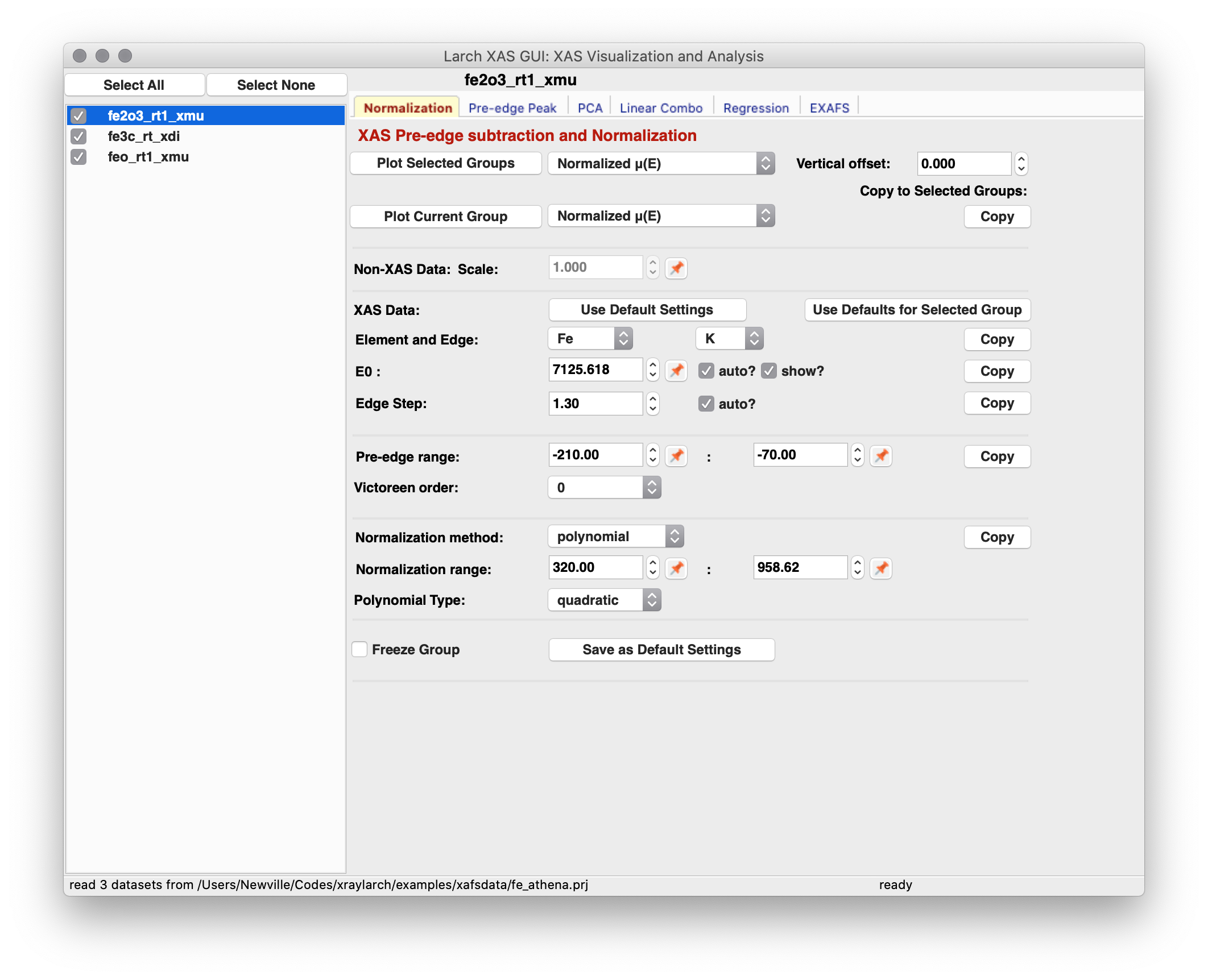
Figure 5.1 XASViewer showing the File/Group list on the left-hand side and the the XAFS pre-edge subtraction and normalization panel on the right.
The right-hand portion of the XAS Viewer window shows multiple forms for more specialized XAFS data processing tasks, each on a separate Notebook tab. These will be covered in more detail in sections below. The default panel shown is for pre-edge subtraction and normalization (Pre-edge subtraction and Normalization), with other available tabs for fitting pre-edge peaks (Pre-edge peak fitting), Linear Combination Analysis (Linear Combination Analysis), Principal Component Analysis (Principal Component and Non-negative Factor Analysis), Advanced Linear Regression (xasviewer_regression), and EXAFS Analysis (EXAFS Processing: Background Subtraction and EXAFS Processing: Fourier Transforms).
There are a few important general notes to mention about XAS Viewer before going into more detail about how to use it. First, XAS Viewer is somewhat new, and in active development. If you find problems with it or unexpected or missing functionality, please let us know. Second, XAS Viewer has many features, functionality, and concepts in common with Athena and Sixpack. This is intentional, as we intend XAS Viewer to be a useful alternative to these applications, possibly with new or better features but also without requiring too much relearning of concepts or workflow. As an important example of this compatibility, XAS Viewer can read in and import data from Athena Project files, and can save these project files as well, so that if you have lots of data organized with Athena Project Files, you can use XAS Viewer and Athena on the same datasets. This aim for compatibility also means that if you find features to be missing or different from how Athena or Sixpack work, let us know.
As a GUI, XAS Viewer is intended to make data processing analysis easy and intuitive. As a Larch application it is also intended to enable more complex analysis, batch processing, and scripting of analysis tasks. To do this, essentially all the real processing work, including most of the plotting of data, in XAS Viewer is done through the Larch Buffer (as shown in Basic Larch GUI) which records the commands that it executes. If, at any point you want to know exactly what XAS Viewer is “really doing”, you can open the Larch Buffer and see the commands being executed. You can also copy the code from the Larch buffer to reproduce the analysis steps, or modify into procedures for batch processing with the Larch scripting language or with Python.
XAS Viewer will display many different datasets as 2-d line plots. As with all such plots made with Larch (see Plotting and Displaying Data), these are highly interactive, customizable, and can produce publication-quality images. The plots can be zoomed in and out, and can be configured to change the colors, linestyles, margins, text for labels, and more. From any plot window you can use Ctrl-C to copy the image to the clipboard, Ctrl-S to Save the image as PNG file, or Ctrl-P to print the image with your systems printer. Ctrl-K will bring up a window with forms to configure the colors, text, styles and so on. These common options are available from the File and Options menu of the plotting window.
In particular, clicking on the legend for any labeled curve on a plot will toggle whether that curve is displayed and partially lighten the label itself. This feature of the plotting window means that XAS Viewer may draw several different traces on the same plot window and allow (or even expect) you to turn some of them on or off interactively to better view the different components being shown. This can be especially useful for comparing XANES spectra or for inspecting the results of peak fitting.
Also note that many of the entries for numbers on the form panels in XAS
Viewer have a button with a ‘pin’ icon ![]() . Clicking anywhere on the
plot window will remember the X and Y values of the last point clicked, and
show the value in the middle section of the status bar, just below the plot
itself. Clicking on any of these ‘pin’ buttons will insert the appropriate
value (usually the energy) from that “most recently clicked position” into
the corresponding field.
. Clicking anywhere on the
plot window will remember the X and Y values of the last point clicked, and
show the value in the middle section of the status bar, just below the plot
itself. Clicking on any of these ‘pin’ buttons will insert the appropriate
value (usually the energy) from that “most recently clicked position” into
the corresponding field.
5.1. Reading Data into XAS Viewer
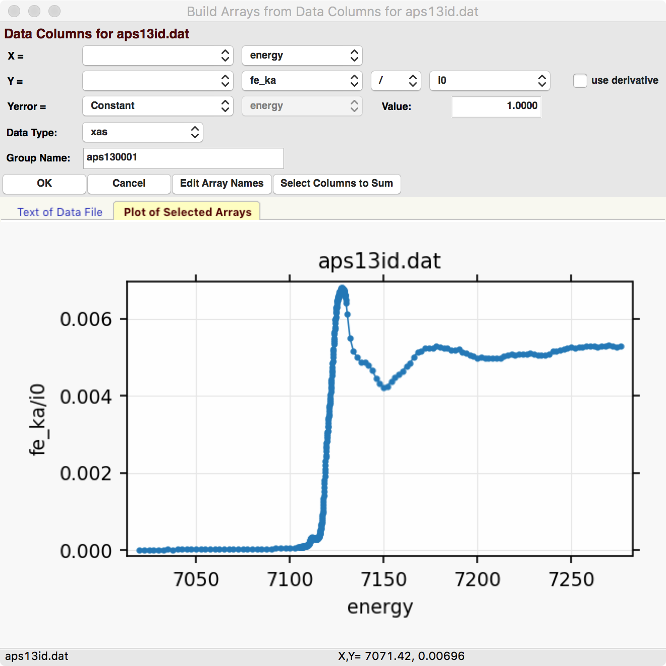
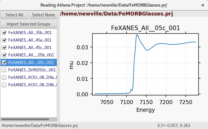
Data groups can be read from plain ASCII data files using a GUI form to help build \(\mu(E)\), or from Athena Project files, as shown in Figure 5.1.1 and Figure 5.1.2. Multiple data groups can be read in, compared, and merged. These datasets can then be exported to Athena Project files, or to CSV files.
When reading in raw data, the data importer shown in Figure 5.1.1 will help you build XAFS \(\mu(E)\) from the various columns in your data file. This form wraps some of the routines described in Chapter Reading and Writing Data. Currently, this form is somewhat limited in being able to process all data formats, but should be useful for many data sets. If you have trouble reading in your data with XAS Viewer, contact us and we will try to help.
5.2. Common XAS Processing Dialogs
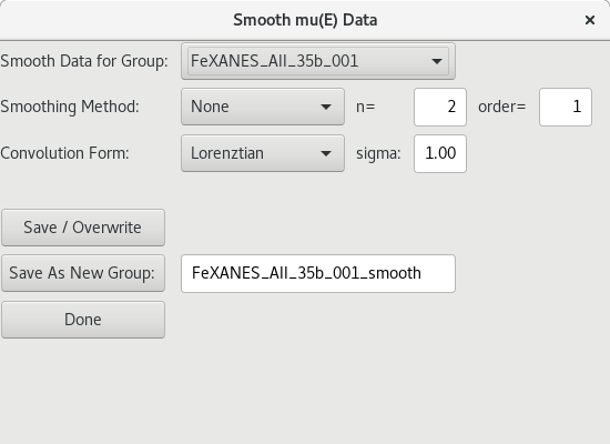
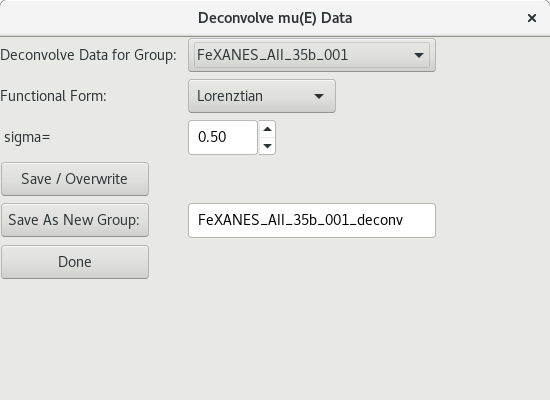
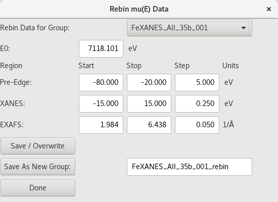
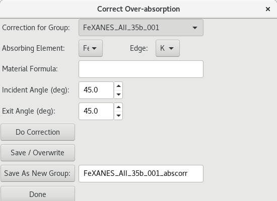
There are several dialogs for interacting with data groups and for doing data corrections. These include speciality dialogs for:
copying, removing, and renaming data groups.
merging of data groups – summing spectra.
de-glitching spectra.
recalibrating spectra.
smoothing of noisy spectra.
re-binning of spectra onto a “normal” XAFS energy grid.
de-convolving spectra.
correcting over-absorption in fluorescence XANES spectra.
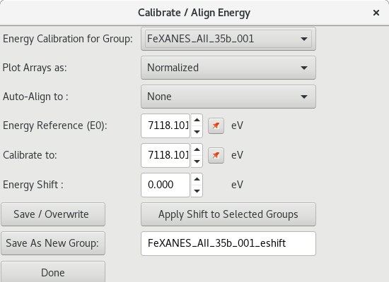
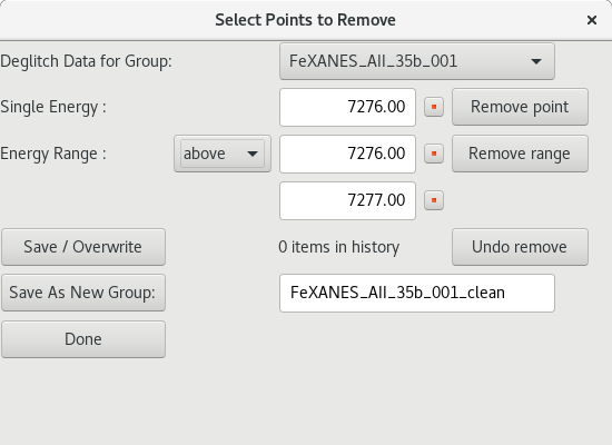
Screenshots of some of these dialogs are shown in the images below.
5.3. Pre-edge subtraction and Normalization
As shown above in Figure 5.1, the main analysis panel for
the XAS Viewer program is the “XAS Normalization” Panel. This panel helps
you do pre-edge subtraction and normalization of XAFS data using the
find_e0(), pre_edge(), or mback_norm() functions. This
processing step is important for getting normalized XAFS spectra that is
used for further analysis of both XANES and EXAFS. In general, the idea is
to get the main step of each XAS spectrum to go from 0 below the main edge
to 1 above the edge, so that the normalized spectrum represents the average
absorption of each absorbing element in the sample.
The first step in the process is to identify \(E_0\), the absorption threshold energy. This is typically (and by default) chosen as the energy point where the first derivative \(d\mu(E)/dE\) has a maximum. This may not necessarily reflect the onset of absorption or the Fermi level, but it is easy to identify reliably for any spectrum. At this point, the value does not have to be highly accurate, so that predictability and reproducibility are favored. You can set the value of \(E_0\) or allow it to be determined automatically.
The next step is to measure how large the jump in absorption is. This
process can be somewhat trickier, so that there are some heuristics built
in to XAS Viewer (and pre_edge()) to help make this more robust.
You can explicitly set the the value of the edge step, or allow it to be
calculated from the spectra in one of two ways.
The classic way for determining the edge step is encapsulated in the
pre_edge() function. Default values for ranges for the fitted
pre-edge line and post-edge normalization curve can be set, or you can rely
on the default settings for these values. In general, the default settings
give pretty good results, but the value for the edge step or the fitting
ranges and curve forms can be altered here.
Consult with pre_edge() and mback_norm() function for more
details on these parameters. Note that you can copy processing parameters
from one group to other groups with the set of “copy” buttons that will
copy the corresponding parameters to all the selected groups.
Finally, from the normalization panel, you can plot the data for the one currently selected group or for all selected groups in a few different ways: Raw \(\mu(E)\), normalized \(\mu(E)\), the derivative \(d\mu(E)/dE\), flattened \(\mu(E)\). For the current group there are even mor options, including the raw \(\mu(E)\) with the pre-edge line and post-edge normalization curve, or compare with the MBACK-calculation for normalization.
5.4. Pre-edge peak fitting
The “Pre-edge Peak Fit” tab (show in Figure 5.4.1) provides a
form for fitting pre-edge peaks to line shapes such as Gaussian, Lorentzian,
or Voigt functions. This provides an easy-to-use wrapper around lmfit
and the minimize() function for curve-fitting with the ability to
constrain fitting Parameters.
Fitting of pre-edge peaks with this panel is a two step process.
First, one fits a “baseline” curve to account for the main absorption edge. This baseline is modeled as a Lorentzian curve plus a line which should be a reasonable enough approximation of the main absorption edge (say, \(4p\)) so that its tail represents the background of the main edge underneath the pre-edge peaks.
Fitting the baseline requires identifying energy ranges for both the main spectrum to be fitted and the pre-edge peaks – the part of the spectrum which should be ignored when fitting the baseline. This is illustrated in Figure 5.4.1 and Figure 5.4.2. Note that there are separate ranges for the “fit range” and the “pre-edge peak” range (illustrated with grey lines and blue circles on the plot). The “pre-edge peak” range should be inside the fit range so that the baseline can fit part of the pre-edge region, at energies below the pre-edge peaks, and part of the main absorption edge region above the pre-edge peaks.
Clicking “Fit baseline” will fit a baseline function and display the plot
as shown below. The initial fit may have poorly guessed ranges for the
pre-edge peaks and fit range and may require some adjustment. As mentioned
above, clicking on the plot will select an energy that can then be
transferred to any of the bounds energy using the corresponding pin icon
![]() on the form.
on the form.
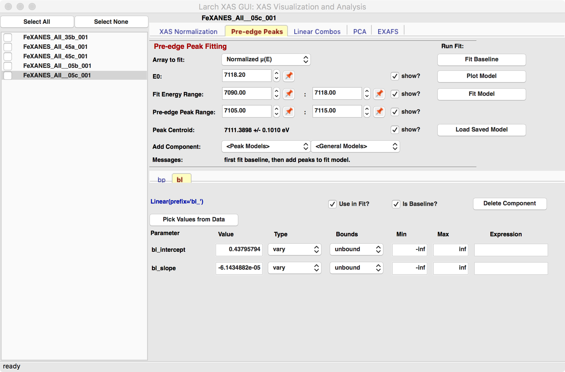
Figure 5.4.1 Pre-edge peak Panel of XASViewer, showing how select regions of pre-edge peaks for fitting a baseline.
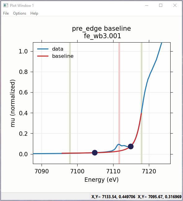
Figure 5.4.2 Plot of pre-edge peaks with baseline. The grey vertical lines show the fit range and blue circles show the boundaries of the pre-edge peak range ignored in the baseline fit. The pink line shows the centroid of the pre-edge peaks after removal of the baseline.
We will allow the baseline to be refined when fitting the peaks, so it does not need to be modeled perfectly, but it is helpful to get a decent fit to the baseline. Once this baseline is satisfactorily modeled, you can add functions to model the pre-edge peaks themselves. Selecting one of the “Peak Models” (typically Gaussian, Lorentzian, or Voigt) will show a new tab in the “model components area” in the lower part of the form. Since the baseline consists of a Lorentzian curve and a line, there will now be 3 tabs for the 3 components of the pre-edge peak model. The background peak and the background line will have tabs labeled bp_ and bl_, respectively, and the added Gaussian curve will be labeled gauss1_, as shown in Figure 5.4.3, which shows the form with 1 Gaussian peak, and the two-component baseline. You can add more peaks by repeatedly selecting the peak type from the drop-down menu labeled Add Component.
Each of the tab for each functional component of the model will include a table of the Parameters for that peak. For example, a line will have an intercept and a slope parameter, and most peak functions will have an amplitude, center, and sigma parameters (and perhaps more). Each of these parameters will have a name and a value, and also have a Type drop-down list to allow it to vary or stay fixed in the fit. You can also set it to be constrained by a simple mathematical expression of other parameter values. If varied, you can also set bounds on the parameter values by using the Bounds drop-down list (to select positive, negative, or custom) and/or set Min and Max values.
After selecting a functional form for the peak, clicking on the “Pick Values from Data” button, and then clicking two points on the plot near the peak of interest will fill in the form with initial values for the parameters for that peak. This is shown in Figure 5.4.3 which has values filled in from the “two click method”, and in Figure 5.4.4 which shows the initial Gaussian peak. The points you pick do not have to be very accurate, and the initial values selected for the amplitude, center, and sigma parameters can be modified. You can also set bounds on any of these parameters – it is probably a good idea to enforce the amplitude and sigma to be positive, for example. If using multiple peaks, it is often helpful to give realistic energy bounds for the center of each peak, so that the peaks don’t try to exchange.
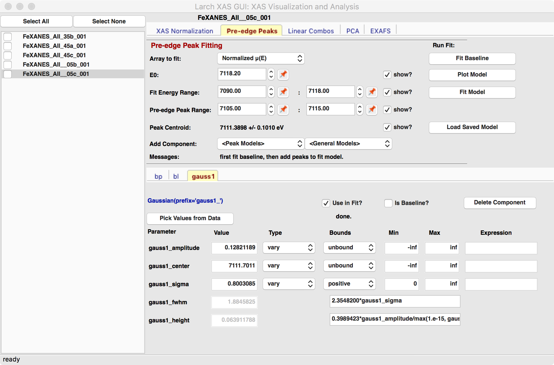
Figure 5.4.3 Pre-edge peak Window of XASViewer, showing 3 components of a Gaussian and a baseline that includes a line and Lorentzian.
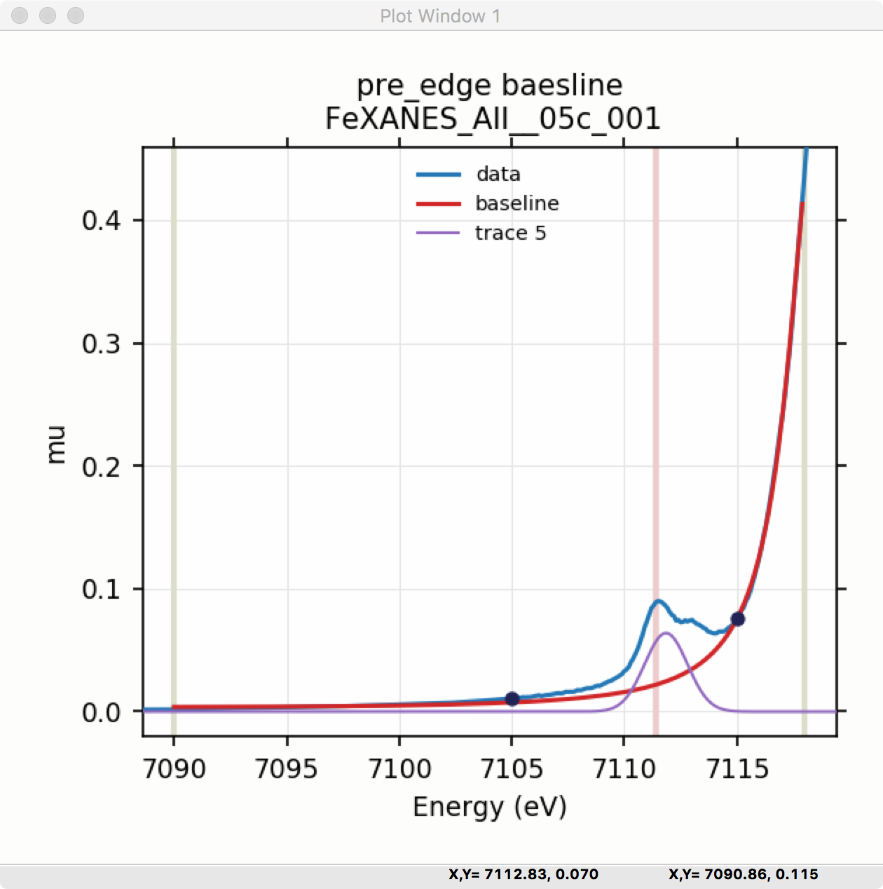
Figure 5.4.4 Plot of initial Gaussian guessed from the “two click method” for modeling pre-edge peaks.
Once the model function is defined and initial parameters values set, clicking the Fit Model button will perform the fit. This will bring up a Fit Result form shown in Figure 5.4.5 and an initial plot of the data and fit as shown in Figure 5.4.6.
The Fit Result panel contains goodness-of-fit statistics and parameter values and uncertainties (or standard error). At the top portion of the form, you can save a model to be read in and used later or export the data and fit components to a simple column-based data file. You can also view the fit goodness-of-fit statistics for the fit. There are also some options and a button for the plot of data and fit.
In the lower portion of the form, you can read the values and uncertainties for the fitting parameters and for a number of derived parameters, including fit_centroid that is the (area-weighted) centroid of the functions that comprise the pre-edge peaks (not including the baseline) and the full-width-at-half-maximum and height of each of the peaks (note that amplitude represents the area of the unit-normalized peak and height represents the maximum height for a peak). You can click on the button labeled “Update Model with these Values” to put these best-fit values back into the starting values on the main form. In addition, clicking on any variable parameter to show it correlations with other variables. Note that the baseline parameters are refined (by default) in the fit to the pre-edge peaks.
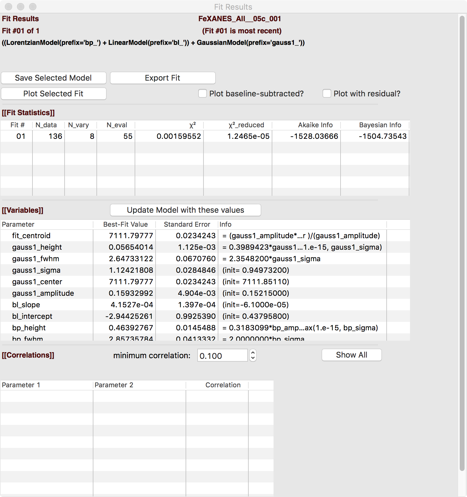
Figure 5.4.5 Fit result frame for Pre-edge peak fit for a fit with 1 Gaussian.
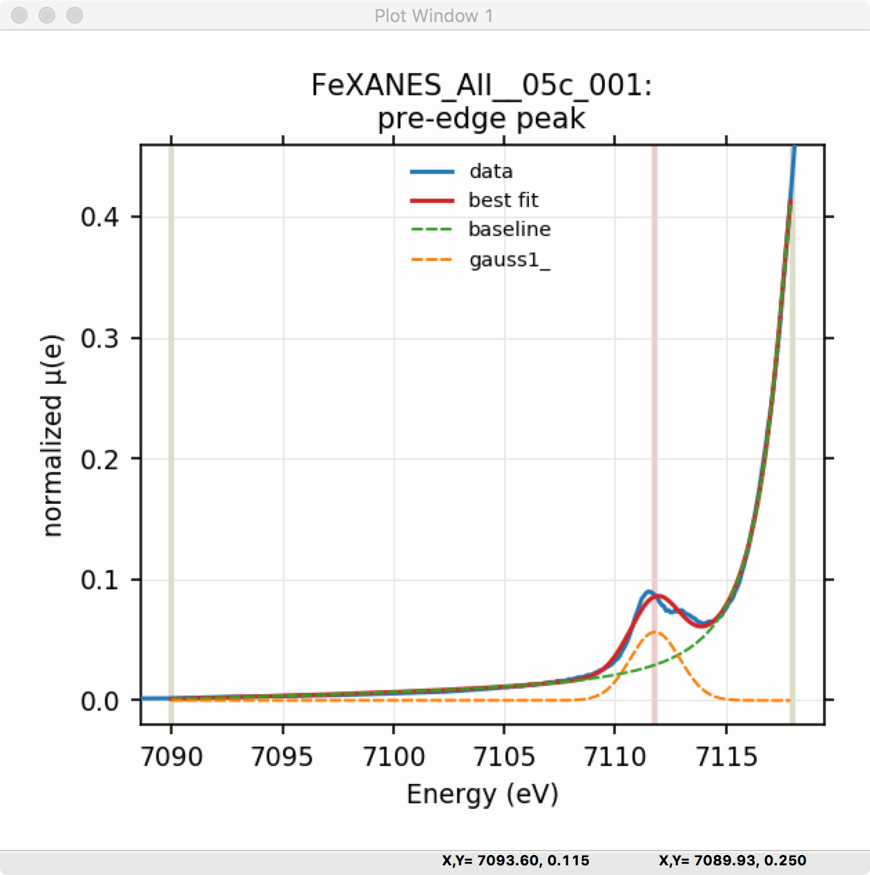
Figure 5.4.6 Pre-edge Peak data and best-fit with 1 Gaussian and baseline.
Though the plot of the fit in Figure 5.4.6 does not look too bad, we can see the fit is not perfect. Checking the “Plot with residual?” box we get the plot in Figure 5.4.7 that shows the data and fit and also the residual. From this, we can see systematic oscillations in the fit residual that is well above the noise level and suggests that another peak may be needed to explain this data. This is not too surprising here – there are obviously two peaks in the pre-edge – but it is does illustrate a useful way to determine when it is useful to add more peaks.
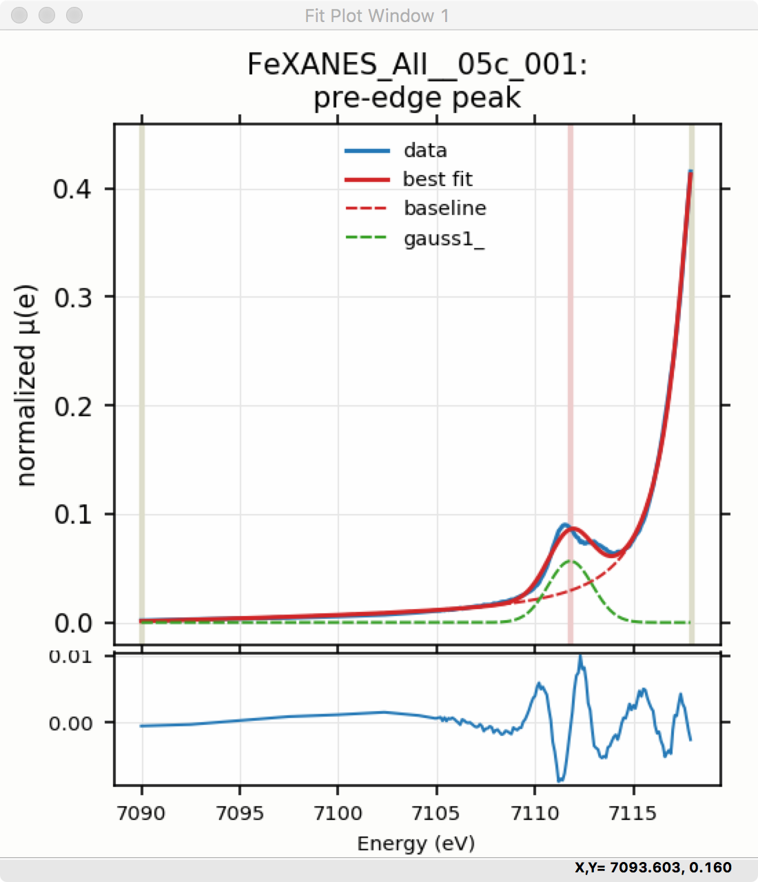
Figure 5.4.7 Pre-edge Peak plot of data, fit and residual.
Adding a second Gaussian (and maybe even a third) will greatly help this fit. If we add another Gaussian peak component to the fit model using the drop-down menu of “Add component:”, select initial values for that second Gaussian before, and re-run the fit, we’ll see the Fit Results form and plot as shown in Figure 5.4.8 and Figure 5.4.9.
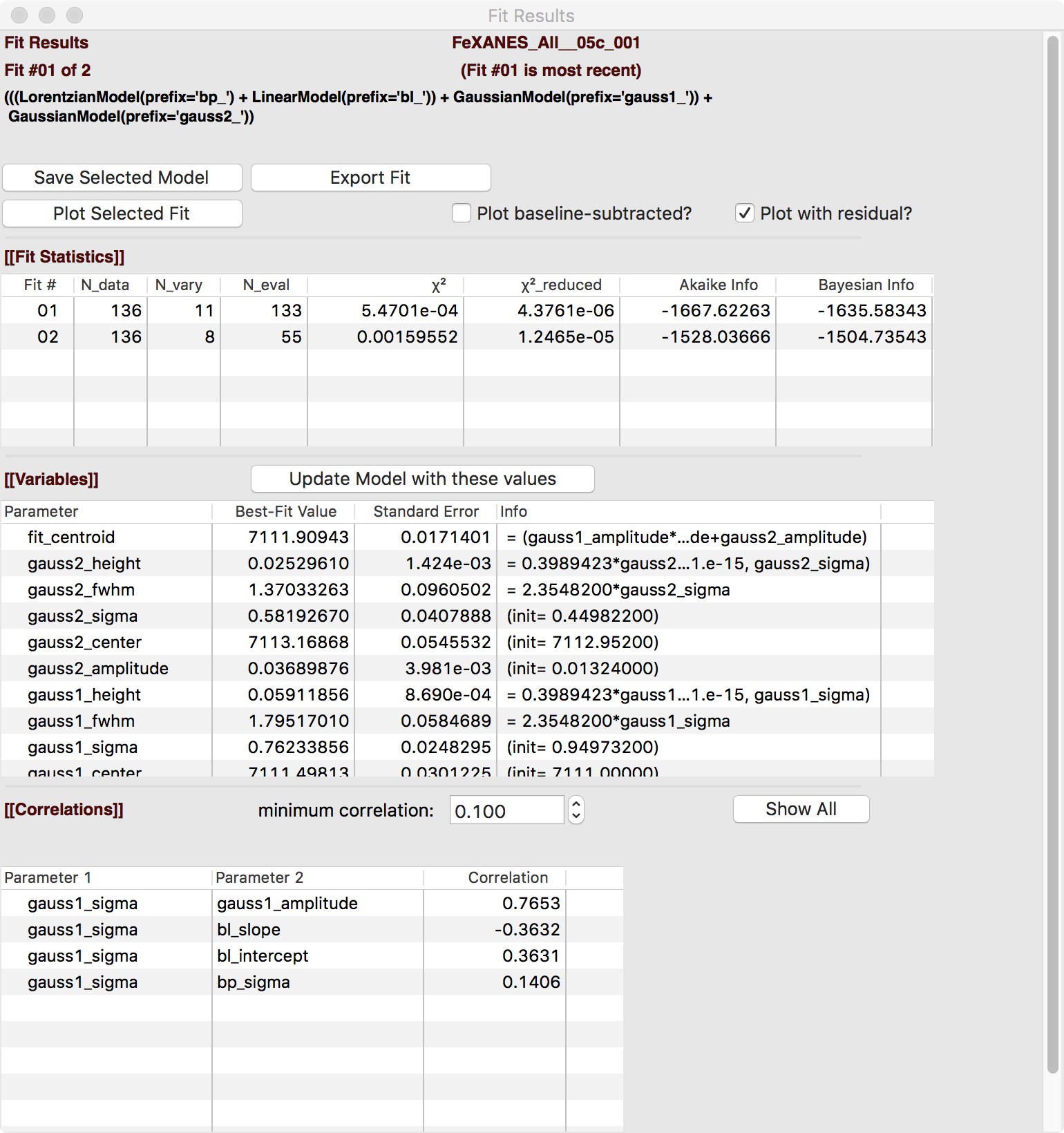
Figure 5.4.8 Fit result frame for Pre-edge peak fit for a fit with 2 Gaussians.
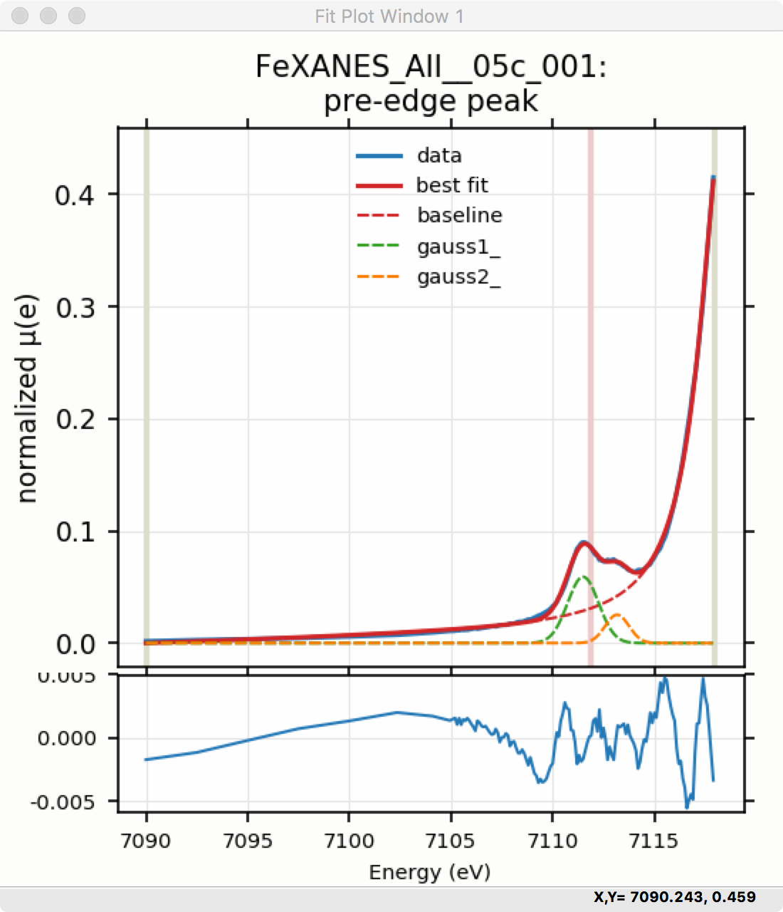
Figure 5.4.9 Pre-edge Peak data and best-fit with 2 Gaussians and baseline.
As mentioned above, fit results can be saved in two different ways, using the “PreEdge Peaks” menu. First, the model to set up the fit can be saved to a .modl file and then re-read later and used for other fits. This model file can also be read in and used with the lmfit python module for complete scripting control. Secondly, a fit can be exported to an ASCII file that will include the text of the fit report and columns including data, best-fit, and each of the components of the model.
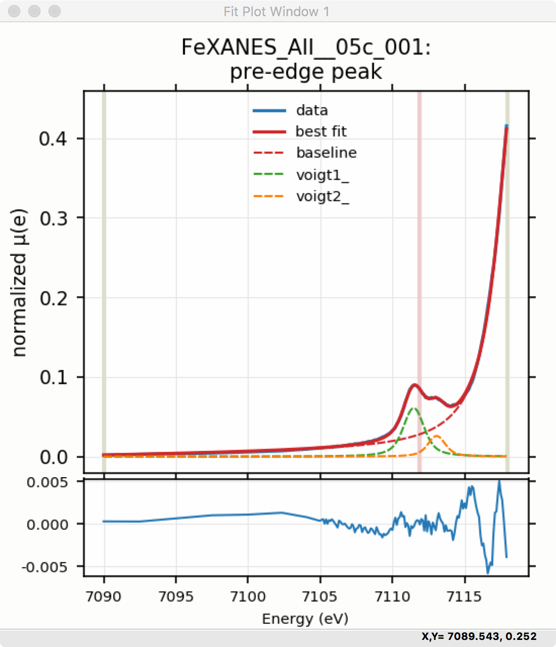
To continue with the analysis of the data in this example, Figure 5.4.9 shows that the fit residual still has significant structure, indicating that either another peak should be included or that the Gaussian peak shape is not a good model for these peaks. In fact, using 2 Voigt functions significantly improves the fit, as shown in Figure 5.4.10, with reduced \(\chi^2\) dropping from 4.4e-6 to 3.2e-6 and similar improvements in the AIC and BIC statistics. To do this, the two Gaussian peaks were deleted and two Voigt peaks added, with initial values selected with the “two click method”.
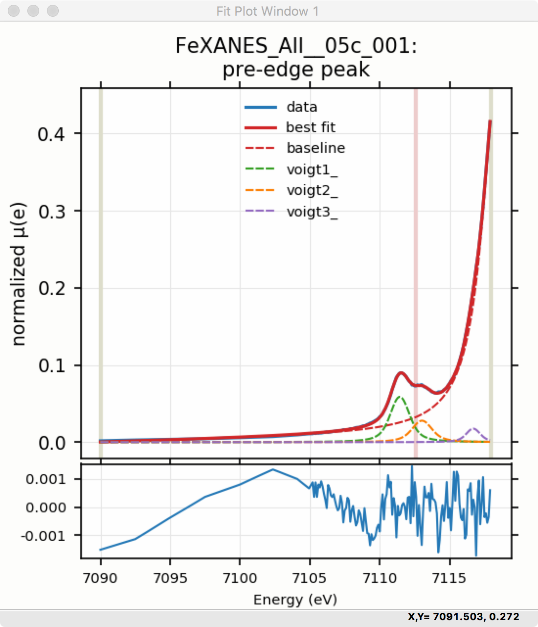
The fit of the pre-edge peaks is visibly improved but a systematic variation in the residual is still seen at the high energy side of the pre-edge peaks. Adding a third Voigt function at around 7117 eV improves the fit even more as shown in Figure 5.4.11. As shown, the scale of the residual is now 0.001, ten times better than the scale of the fit with 1 peak shown in Figure 5.4.7, and shows much less systematic structure. In addition, all the fit statistics are improved despite now using 14 variables: reduced \(\chi^2\) becomes from 5.1e-7, AIC is -1957 and BIC is -1917.
5.5. Linear Combination Analysis
Linear Combination Analysis is useful for modeling a XANES spectrum as a combination of other spectra.
5.6. Principal Component and Non-negative Factor Analysis
Principal Component Analysis (PCA) is one of a family of numerical techniques to reduce the number of variable components in a set of data. There are many related techniques and procedures, and quite a bit of nomenclature and jargon around the methods.
In essence, all these methods are aimed at taking a large set of similar data and trying to determine how many independent components make up that larger dataset. That is, the only question PCA and related methods can ever really answer is:
how many independent spectra make up my collection of spectra?
It is important to note that PCA cannot tell you what those independent spectra represent or even what they look like. However, you can also use the results of PCA to ask:
is this *other* spectrum made up of the same components as make up my collection?

