13.7. Simplified Peak Fitting with fit_peak()
As shown in the previous sections, it is pretty simple to use Larch’s
fitting mechanism to set up and perform fits to data. In fact, it is
pretty commom to need to fit data to simple line-shapes, as when setting up
an experiment. In an effort to make life easier, in addition to providing
a fairly easy general-purpose fitting function, Larch provides a
fit_peak() function to fit one dimensional data to one of several
lineshapes.
- _math.fit_peak(x, y, model, dy=None, background=None, step=None, negative=False, use_gamma=False)
fit the data y at points x with a function described by model, optionally including uncertainties in y, a background polynomial, and a choice of step functions.
- Parameters:
x – array of values at which to calculate model
y – array of values for model to try to match
model – name of model for functional form to use. See Table of fit_peak models.
dy – optional array of values for uncertainty in y data to be matched.
background – name of background model to use. One of (case insensitive) None (no background), ‘constant’, ‘linear’, or ‘quadratic’. This is ignored when model is ‘linear’ or ‘quadratic’
step – name of step model to use for ‘step’ and ‘rectangle’ models. One of (case insensitive): ‘linear’, ‘erf’, or ‘atan’
negative – boolean for whether peak or steps are expected to go down (default
False)use_gamma – boolean for whether to use separate gamma parameter for ‘voigt’ model (default
False).
- Returns:
a Group containing fit parameters, best-fit and background functions, as detailed in Table of fit_peak group members.
Table of
fit_peak()models.The following functional models are supported for fitting with
fit_peak().
model
Description
parameter names
linear
\(y = mx + b\)
offset, slope
quadratic
\(y = a + bx + cx^2\)
offset, slope, quad
step
step function
height, center, width
rectangle
step up, step down
height, center1, width1, center2, width2
exponential
\(y = Ae^{-x/b}\)
amplitude, decay
gaussian
Gaussian
amplitude, center, sigma
lorentzian
Lorenztian
amplitude, center, sigma
voigt
Voigt (with gamma=sigma)
amplitude, center, sigma
The sigma and width parameters will have a minimum value of 0.
For all models except linear and quadratic, an optional background can be included, which (depending on the form chosen) will add parameters named bkg_offset, bkg_slope, and bkg_quad.
Table of members of group returned by
fit_peak().
member
Description
x
copied from input x data
y
copied from input y data
model
name of model used
background
name of background models used
step
name of step model used
params
Group of fit parameters, as sent to and from
minimize()fit
final best fit to y data, including background if used.
fit_init
initial guess of fit to y data, including background if used.
bkg
final background function, if used.
bkg_init
initial background function, if used.
13.7.1. Example: Fitting a Gaussian + background with fit_peak()
As in the Example in the previous section, we make a simple mock data set and fit a Gaussian function to it. Here we also add a linear background, and do the whole fit with a single function, instead of a dozen or so lines of code used before:
## examples/fitting/doc_example_fitpeak1.lar
# create mock data
x = linspace(0, 100, 51)
noise = random.normal(size=len(x), scale=0.1)
y = 8.0 - x*0.025 + noise
y = y + voigt(x, amplitude=89.0, center=44.25, sigma=4.75, gamma=2.0)

# fit to Gaussian with linear background
myfit = fit_peak(x, y, 'gaussian', background='linear')

plot(myfit.x, myfit.y, marker='+', label='data',
     xlabel='x', ylabel='y', show_legend=True, new=True)
plot(myfit.x, myfit.fit_init, label='init')
plot(myfit.x, myfit.fit, label='best fit')

print( fit_report(myfit, min_correl=0.3))

## end examples/fitting/doc_example_fitpeak1.lar
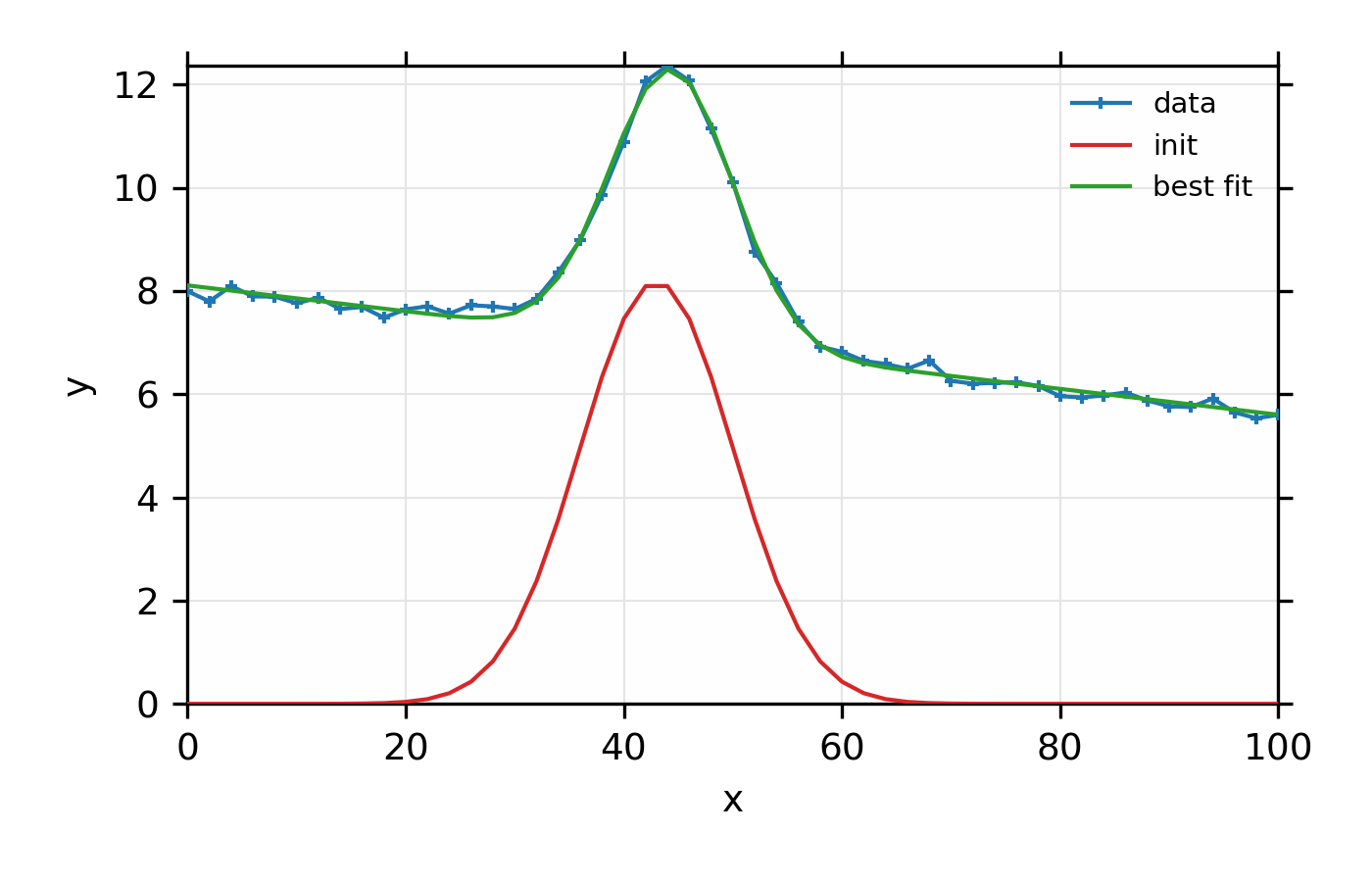
Here we first create mock data that’s fairly noisy, and ask it to be fit to Gaussian, including a linear background, with a single command. We then plot the results and print the report of parameters. Note that the fit is pretty good at finding the peak center and shape, even though the model is not strictly correct.
The printed output from fit_report(myfit) will look like this:
[[Model]]
    (Model(gaussian) + Model(linear, prefix='bkg_'))
[[Fit Statistics]]
    # function evals   = 33
    # data points      = 51
    # variables        = 5
    chi-square         = 0.62209
    reduced chi-square = 0.013524
    Akaike info crit   = -214.73
    Bayesian info crit = -205.07
[[Variables]]
    amplitude:       75.4295207 +/- 1.085962 (1.44%) (init= 143.506)
    bkg_intercept:   8.10849304 +/- 0.035243 (0.43%) (init= 0)
    bkg_slope:      -0.02506582 +/- 0.000562 (2.24%) (init= 0)
    center:          44.3598293 +/- 0.079202 (0.18%) (init= 43)
    fwhm:            13.3776066 +/- 0.198318 (1.48%)  == '2.3548200*sigma'
    height:          5.29700921 +/- 0.065021 (1.23%)  == 0.3989423*amplitude/max(1.e-15, sigma)'
    sigma:           5.68094659 +/- 0.084218 (1.48%) (init= 7)
[[Correlations]] (unreported correlations are <  0.300)
    C(bkg_intercept, bkg_slope)  = -0.835
    C(amplitude, sigma)          =  0.647
    C(amplitude, bkg_intercept)  = -0.402
And the plot of data and fit will look like this:

Figure 13.7.1.1 Simple fit to mock data using a Gaussian model and a linear background
with the fit_peak() function.
Although the fit is quite good, the model is probably imperfect, and using a Voigt function to fit to this data would give better results. The main point here is not just that the fit is good, but that it was accomplished with a single line of code.
13.7.2. Example: Fitting a Rectangular function with fit_peak()
Here, we simulate data that might represent a line-up scan at a beamline. The fit is to a function that takes a step up and a step down.
## examples/fitting/doc_example_fitpeak2.lar
# create mock rectangular data
def make_rect_data(x, noise_scale=0.01):
    noise = random.normal(size=len(x), scale=noise_scale)
    y = 6.0 - x*0.001 + noise
    x0 = 30
    dx = 7
    sig = dx*0.6
    y = y + gaussian(x, amplitude=68, center=x0+0*dx, sigma=1.2*sig)
    y = y + gaussian(x, amplitude=60, center=x0+1*dx, sigma=1.1*sig)
    y = y + gaussian(x, amplitude=71, center=x0+2*dx, sigma=sig)
    y = y + gaussian(x, amplitude=75, center=x0+3*dx, sigma=sig)
    y = y + gaussian(x, amplitude=70, center=x0+4*dx, sigma=sig)
    y = y + gaussian(x, amplitude=65, center=x0+5*dx, sigma=sig)
    y = y + gaussian(x, amplitude=72, center=x0+6*dx, sigma=sig)
    y = y + gaussian(x, amplitude=61, center=x0+7*dx, sigma=0.9*sig)
    return y
#enddef

x = linspace(0, 160, 321)
y = make_rect_data(x, noise_scale=0.2)

# fit to rectangle shape
myfit = fit_peak(x, y, 'rectangle', background='constant', step='erf')

plot(myfit.x, myfit.y, marker='+', label='data',
     xlabel='x', ylabel='y', show_legend=True, new=True)
plot(myfit.x, myfit.fit, label='best fit')

print( fit_report(myfit, min_correl=0.3))

## end examples/fitting/doc_example_fitpeak2.lar
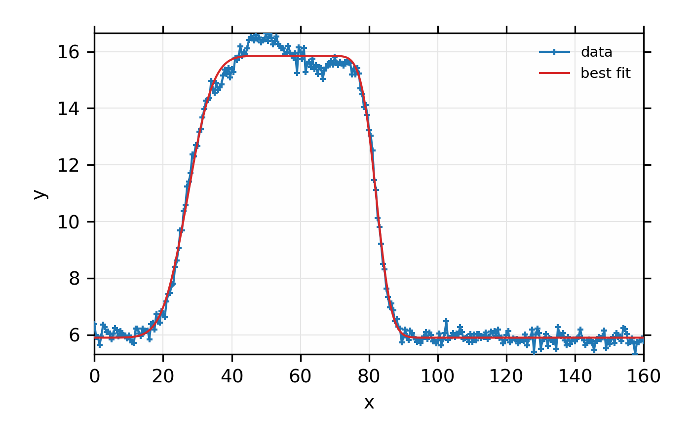
Again, we first create mock data that’s fairly noisy. The data is clearly
not exactly rectangular, but we ask it to be fit to a rectangular function
plus a linear background. The printed output from fit_report(myfit)
will look like this:
[[Model]]
    (Model(rectangle, form='erf') + Model(constant, prefix='bkg_'))
[[Fit Statistics]]
    # function evals   = 67
    # data points      = 321
    # variables        = 6
    chi-square         = 23.405
    reduced chi-square = 0.074301
    Akaike info crit   = -828.54
    Bayesian info crit = -805.91
[[Variables]]
    amplitude:   9.95178246 +/- 0.038770 (0.39%) (init= 11.34094)
    bkg_c:       5.90041256 +/- 0.020680 (0.35%) (init= 0)
    center1:     27.1354829 +/- 0.095553 (0.35%) (init= 26.5)
    center2:     82.0689673 +/- 0.071565 (0.09%) (init= 81.5)
    midpoint:    54.6022251 +/- 0.055873 (0.10%)  == '(center1+center2)/2.0'
    sigma1:      8.14570023 +/- 0.186184 (2.29%) (init= 32)
    sigma2:      4.88414083 +/- 0.140778 (2.88%) (init= 32)
[[Correlations]] (unreported correlations are <  0.300)
    C(amplitude, bkg_c)          = -0.566
    C(amplitude, sigma1)         =  0.341

Figure 13.7.2.1 Simple fit to mock data to a rectangular function and a linear
background using the fit_peak() function.
Again, the principle point here is not how well the rectangular model matches the actual data here, but how simply one can model data to a selection of simple shapes. Such fits can be very useful for preliminary data visualization and analysis. Of course, one should be cautious about treating the results of such an automated approach as a final and best analysis of any data.
13.7.3. Using lmfit.Model
Note that the fit_peak() function gives a simple wrapping of
lmfit.Model. For a wider selection of builtin
Models and more sophisticated model building including adding bounds and
constraints between parameters one can import and use lmfit.Model directly with larch. As an example, the above fit can be
replicated with:
larch> from lmfit.models import RectangleModel, ConstantModel
larch> model = RectangleModel(form='erf') + ConstantModel(prefix='bkg_')
larch> params = model.make_params(bkg_c=0, sigma1=10, sigma2=10,
                                  center1=20, center20=80, amplitude=10)
larch> out = model.fit(y, params, x=x)
larch> print(out.fit_report(sorted_pars=True))
Here, a model is built as the sum of two components: a rectangle and a
constant background. lmfit.Parameters are made
from this composite model and the parameter names, giving initial values
for each parameter. The model can then be used to fit the data y with
the parameters params, and the independent variable x. While
directly using lmfit.Model does require providing
initial values for all parameters, it also gives complete access to the
parameters, and allows building more complex models.
