13.8. Advanced Confidence Intervals and Chi-square maps
Having good estimates for uncertainties in fitted parameters is important
for any scientific analysis. One of principle attractions to using the
Levenberg-Marquardt algorithm that is the default fitting mechanism with
the minimize() function is that it will automatically calculate
estimates of parameter uncertainties and correlations. This is very
convenient and generally reliable, but it should be made clear that the
basic assumptions made when these uncertainties are estimated are not
always perfect. Unfortunately, it is sometimes difficult to tell when this
is the case.
It is therefore fairly common to see analyses that include explicit exploration of Parameter values away from their best-fit solution, in order to determine the degree of confidence in the best-fit values. Larch provides two main functions to help explore such cases. To be sure, they are much slower than the automatic estimation of the uncertainties. For many (perhaps most) cases, they do not provide much better insight than the automatic method.
- confidence_intervals(minimizer, sigmas=(1, 2, 3), prob_func=None, maxiter=200)
Calculate confidence intervals for the parameters from a given fit.
- Parameters:
minimizer – the minimizer object returned by
minimize().sigmas – list of sigma-levels to find parameter values for.
prob_func –
Noneor callable function to calculate the probability from the optimized chi-square. By default,f_compare(), the standard F-test, is used.
- Returns:
a dictionary of parameter names, with each value containing a list of (sigma, value) pairs.
This function will adjust the value for each parameter, re-optimizing the other parameters until it finds the parameter values that increase sigma by the levels indicated.
- confidence_report(conf_values)
Convert the output of
confidence_intervals()into a printable report.- Parameters:
conf_values – confidence values returned by
confidence_intervals().- Returns:
a string containing the report, which can be printed or stored.
- f_test(ndata, nparams, chisquare, chisquare0, nfix=1)
Returns the standard F-test value for the probability that one fit is better than another.
13.8.1. Confidence interval, Example 1
Let’s begin with a shortened version of the first example from the previous section.
## examples/fitting/doc_example_conf1.lar
# create mock data
mdat = group()
mdat.x = linspace(-10, 10, 201)
mdat.y = 1.0 + gaussian(mdat.x, 12.0, 1.5, 2.0) + \
         random.normal(size=len(mdat.x), scale=0.050)


params = param_group(off = guess(0),
                     amp = guess(5, min=0),
                     cen = guess(2),
                     wid = guess(1, min=0))


# define objective function for fit residual
def myresid(p, data):
    return data.y - (p.off + gaussian(data.x, p.amp, p.cen, p.wid))
#enddef

# perform fit

result = minimize(myresid, params, args=(mdat,))

# print report of parameters, uncertainties
print( fit_report(result))

out = confidence_intervals(result, sigmas=(1, 2, 3))

print( confidence_report(out))
## end of examples/fitting/doc_example_conf1.lar
The printed output from fit_report(params) will include this:
[[Variables]]
   amp            =  12.129867 +/- 0.124722 (init=  5.000000)
   cen            =  1.476822 +/- 0.017266 (init=  2.000000)
   off            =  0.998814 +/- 0.007131 (init=  0.000000)
   wid            =  2.022301 +/- 0.016938 (init=  1.000000)

[[Correlations]]     (unreported correlations are <  0.100)
   amp, off             = -0.861
   amp, wid             =  0.808
   off, wid             = -0.692
=======================================================
while the output from the much more explicit search done in
confidence_intervals() and reported by confidence_report() will be:
# Confidence Interval Report
# Sigmas:          -3         -2         -1          0          1          2          3
# Percentiles:  -99.730    -95.450    -68.269      0.000     68.269     95.450     99.730
#==========================================================================================
 amp             11.755      11.88     12.005      12.13     12.256     12.385     12.517
    -best      -0.37459   -0.24967   -0.12455          0    0.12604    0.25555    0.38759
 wid             1.9707     1.9885     2.0053     2.0223     2.0395     2.0569     2.0749
    -best     -0.051552  -0.033784  -0.016975          0   0.017156   0.034567   0.052626
 off             0.9766    0.98468     0.9912    0.99881     1.0064     1.0128     1.0209
    -best     -0.022212  -0.014138  -0.0076156          0  0.0075667   0.013987   0.022049
 cen             1.4248     1.4423     1.4596     1.4768     1.4941     1.5113     1.5289
    -best     -0.052057   -0.03452  -0.017248          0   0.017249   0.034524   0.052068
The automatic error estimates given from minimize() are meant to be
1-\(\sigma\) uncertainties. Comparing the two methods we find:
Parameter
Best Value
Automatic 1-\(\sigma\) value
Explicit 1-\(\sigma\) value
amp
12.1299
+/- 0.1247
+0.1267, -0.1246
cen
1.4768
+/- 0.0173
+0.0172, -0.0172
off
0.9988
+/- 0.0071
+0.0076, -0.0076
cen
2.0223
+/- 0.0169
+0.0172, -0.0170
which seems to justify the use of the automated method. The uncertainties found from the more thorough exploration shows symmetric uncertainties, even out to the 3-\(\sigma\) level, and of the 4 1-\(\sigma\) uncertainties, 3 are within 2%, and the worst agreement, for the smallest uncertainty is within 7%. It also shows that the scaling of uncertainties is fairly linear with \(\sigma\): the 3-\(\sigma\) values are approximately 3 times the 1-\(\sigma\) values.
13.8.2. Confidence interval, Example 2
Of course, there are more challenging cases than the one above. A double exponential function is one such example, so we start with a fit to mock data
## examples/fitting/doc_example_conf2.lar
#  Shows usage of fitting with non-normal correlation of variables,
#  and confidence intervals.

random.seed(1)
dat = group(x = linspace(0, 10, 101))
dat.y = 3*exp(-dat.x/2) - 5*exp(-dat.x/9) + random.normal(size=len(dat.x), scale=0.05)

fitparams = param_group(a1 = guess(3.5),
                        a2 = guess(-9.5),
                        t1 = guess(3),
                        t2 = guess(15))

def fit_exp(pars, dat):
    model = pars.a1 * exp(-dat.x / pars.t1) + pars.a2 * exp(-dat.x / pars.t2)
    return model - dat.y
enddef

minout = minimize(fit_exp, fitparams, args=(dat,))
print( fit_report(minout, min_correl=0))

final = fit_exp(fitparams, dat) + dat.y
newplot (dat.x, dat.y, label='data', marker='o', linewidth=0)
   plot (dat.x, final, label='fit')

## end of examples/fitting/doc_example_conf2.lar
The resulting statistics report with the automated uncertainties is:
===================== FIT RESULTS =====================
[[Statistics]]    Fit succeeded,  method = 'leastsq'.
   Message from fit    = Fit succeeded.
   npts, nvarys, nfree = 101, 4, 97
   nfev (func calls)   = 36
   chi_square          = 0.191322
   reduced chi_square  = 0.001972

[[Variables]]
   a1             =  2.828857 +/- 0.149776 (init=  3.500000)
   a2             = -4.819553 +/- 0.159495 (init= -9.500000)
   t1             =  1.878519 +/- 0.100212 (init=  3.000000)
   t2             =  9.270866 +/- 0.309035 (init=  15.000000)

[[Correlations]]     (unreported correlations are <  0.100)
   a2, t2               =  0.991
   a1, a2               = -0.991
   a1, t2               = -0.988
   a2, t1               = -0.968
   t1, t2               = -0.937
   a1, t1               =  0.935
=======================================================
You can see that the correlations between all 6 pairs of variables is above 90%. The resulting plot of the best-fit looks fairly reasonable:
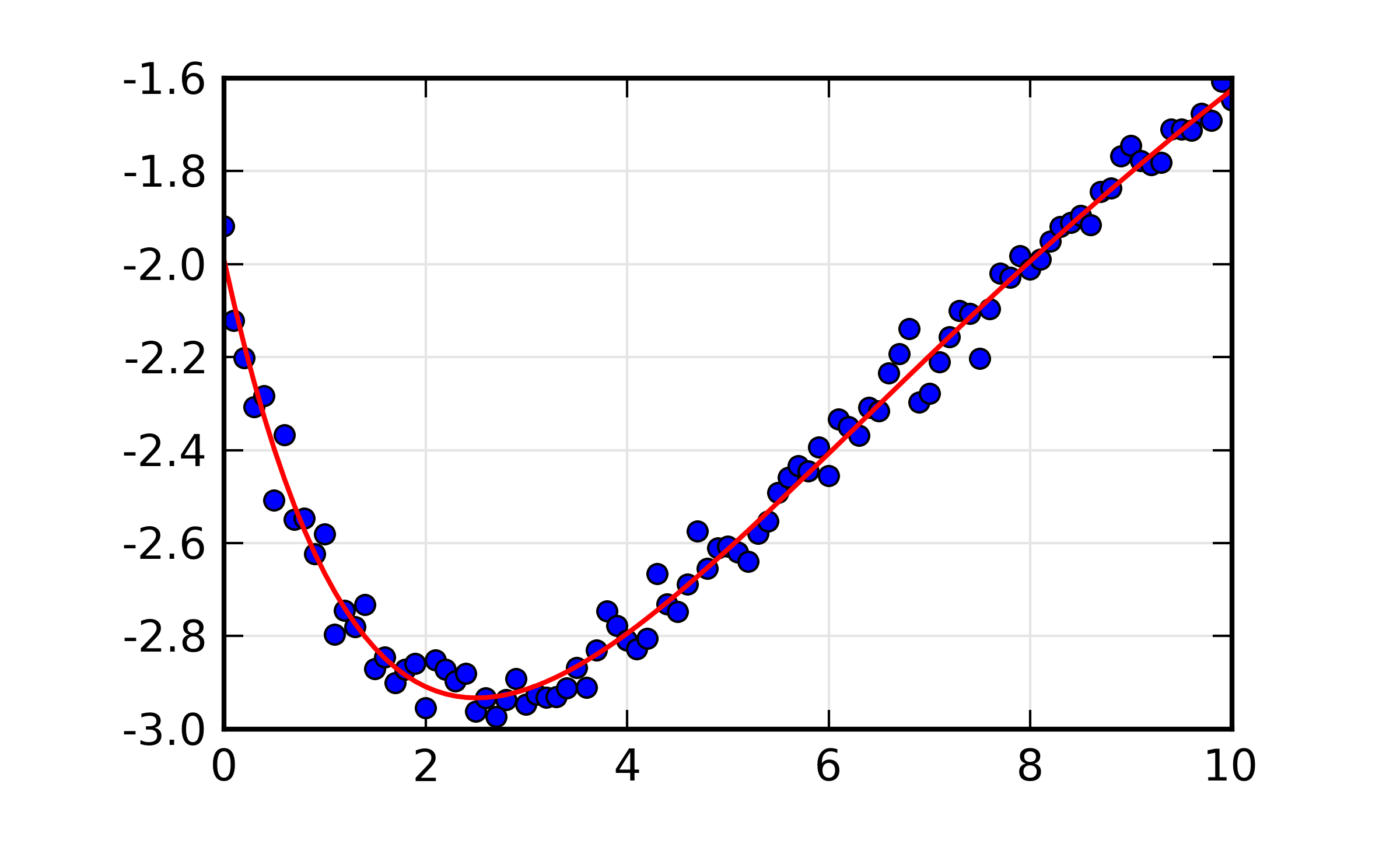
Figure 13.8.2.1 Fit to double exponential function.
But if we we ask for the more thorough investigation of the confidence intervals in these parameters with:
conf_int = confidence_intervals(minout)
print confidence_report(conf_int)
the resulting report is:
# Confidence Interval Report
# Sigmas:          -3         -2         -1          0          1          2          3
# Percentiles:  -99.730    -95.450    -68.269      0.000     68.269     95.450     99.730
#==========================================================================================
 a1              2.4622     2.5704      2.691     2.8289     2.9936     3.1985      3.467
    -best      -0.36665   -0.25842   -0.13785          0    0.16472    0.36968    0.63812
 a2             -5.4926    -5.2111    -4.9945    -4.8196    -4.6726     -4.544     -4.429
    -best      -0.67309   -0.39152   -0.17499          0    0.14698    0.27553    0.39058
 t2              8.2604     8.6221     8.9556     9.2709     9.5761     9.8776     10.182
    -best       -1.0105   -0.64882   -0.31531          0    0.30526    0.60676    0.91132
 t1              1.6107     1.6942     1.7827     1.8785     1.9841     2.1049     2.2456
    -best      -0.26785   -0.18436   -0.09583          0    0.10553    0.22637    0.36709
Now can see more asymmetric uncertainty values, specifically that the -n-\(\sigma\) and +n-\(\sigma\) are different, and don’t seem to be linear in n. Comparing the 1-\(\sigma\) levels between the automated and explicit methods as we did above, we now have
Parameter
Best Value
Automatic 1-\(\sigma\) value
Explicit 1-\(\sigma\) value
a1
2.8289
+/- 0.1498
+0.1647, -0.1379
a2
-4.8196
+/- 0.1595
+0.1470, -0.1750
t1
9.2709
+/- 0.1002
+0.1055, -0.0958
t2
1.8785
+/- 0.3090
+0.3053, -0.3153
In fairness, the automated values don’t look too bad, given that they cannot reflect asymmetric uncertainties. But, like the reported correlations, the full report above hints at a less than ideal case.
13.8.3. Chi-square Maps
We can further explore the correlation between pairs of variables by making
and visualizing a map of the chi-square (\(\chi^2\)) statistic. This
can be helpful to determine if the automatically calculated uncertainties
and correlation are reasonable, and to look for pathological cases. The
chi2_map() function will calculate a map of \(\chi^2\) for a pair
of variable parameters by brute force.
- chi2_map(minimizer, xname, yname, nx=11, ny=11, sigmas=5, xrange=None, yrange=None)
Return a chi-square map for two parameters in a fit
- Parameters:
minimizer – the minimizer object returned by
minimize().xname – name of variable for x-axis
yname – name of variable for y-axis
nx – number of steps in x [11]
ny – number of steps in y [11]
sigmas – extent of x, y values to calculate, in \(\sigma\)
xrange – explicit x range of calculations [x.best +/-
sigmas* x.stderr]yrange – explicit y range of calculations [y.best +/-
sigmas* y.stderr]
- Returns:
a tuple of (x_vals, y_vals, chi2_map)
The
xrangeandyrangearguments can be used to fully dictate the x and y values to use. By default, the x and y values are automatically determined fromnx,ny, andsigmas, with thesigmasargument sets how far from the best value to extend the ranges.
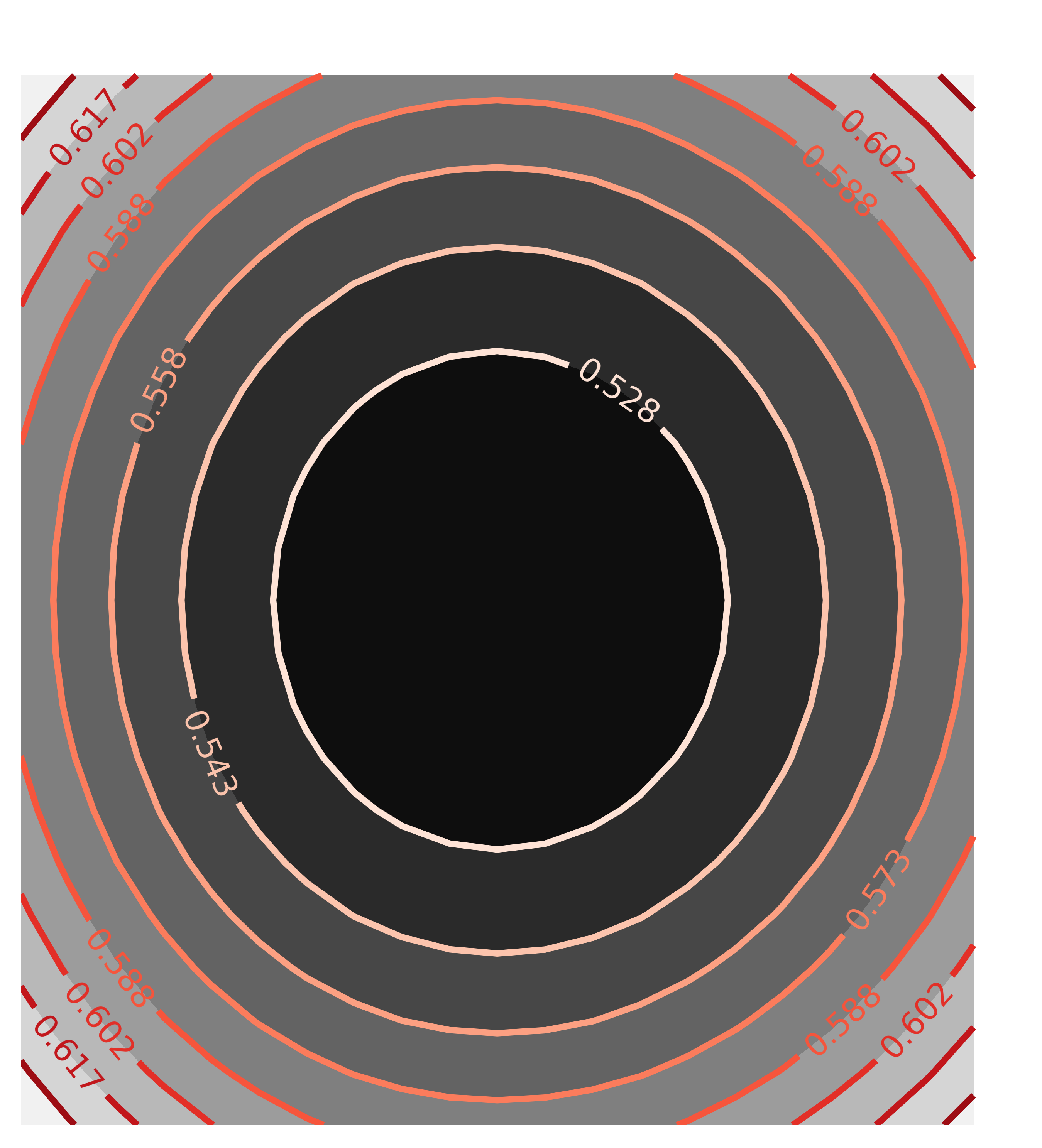
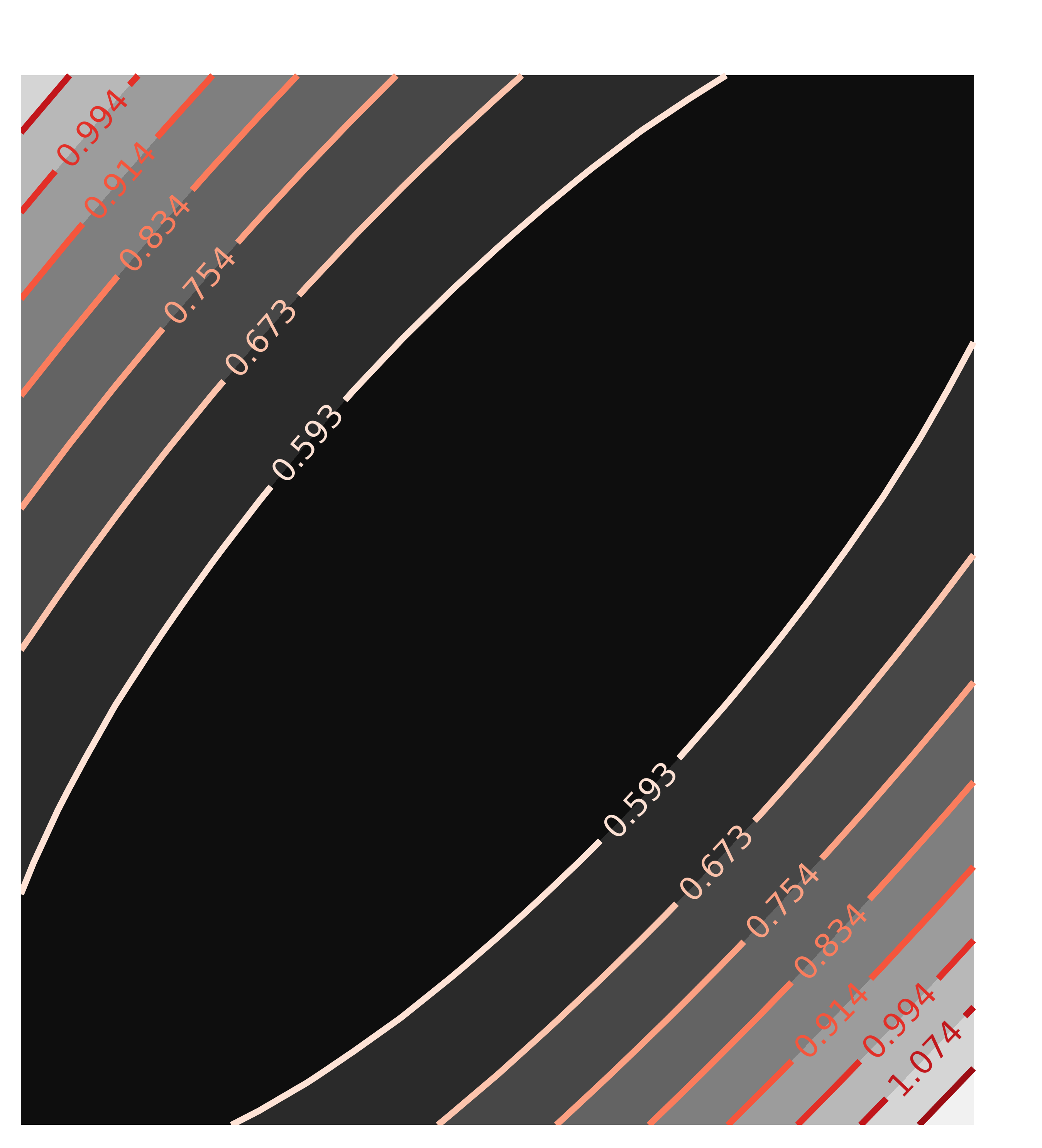
As an example usage, we return to the first example of the “well-behaved”
fit, and run chi2_map() on a pair of variables with low correlation
and a pair with high correlation:
x1, y1, chi2_ampcen = chi2_map(mout, 'amp', 'cen', nx=21, ny=21)
x2, y2, chi2_ampwid = chi2_map(mout, 'amp', 'wid', nx=21, ny=21)
contour(chi2_ampcen, x=x1, y=y1, title='Correlation(amp, cen)')
contour(chi2_ampwid, x=x2, y=y2, win=2, title='Correlation(amp, wid)')
with the resulting Chi-square maps looking like this:
The circular map for the uncorrelated parameters amp and cen and the elliptical map for the highly correlated parameters amp and wid are exactly as would be expected, and what the automated estimate of uncertainties and correlations assumes.
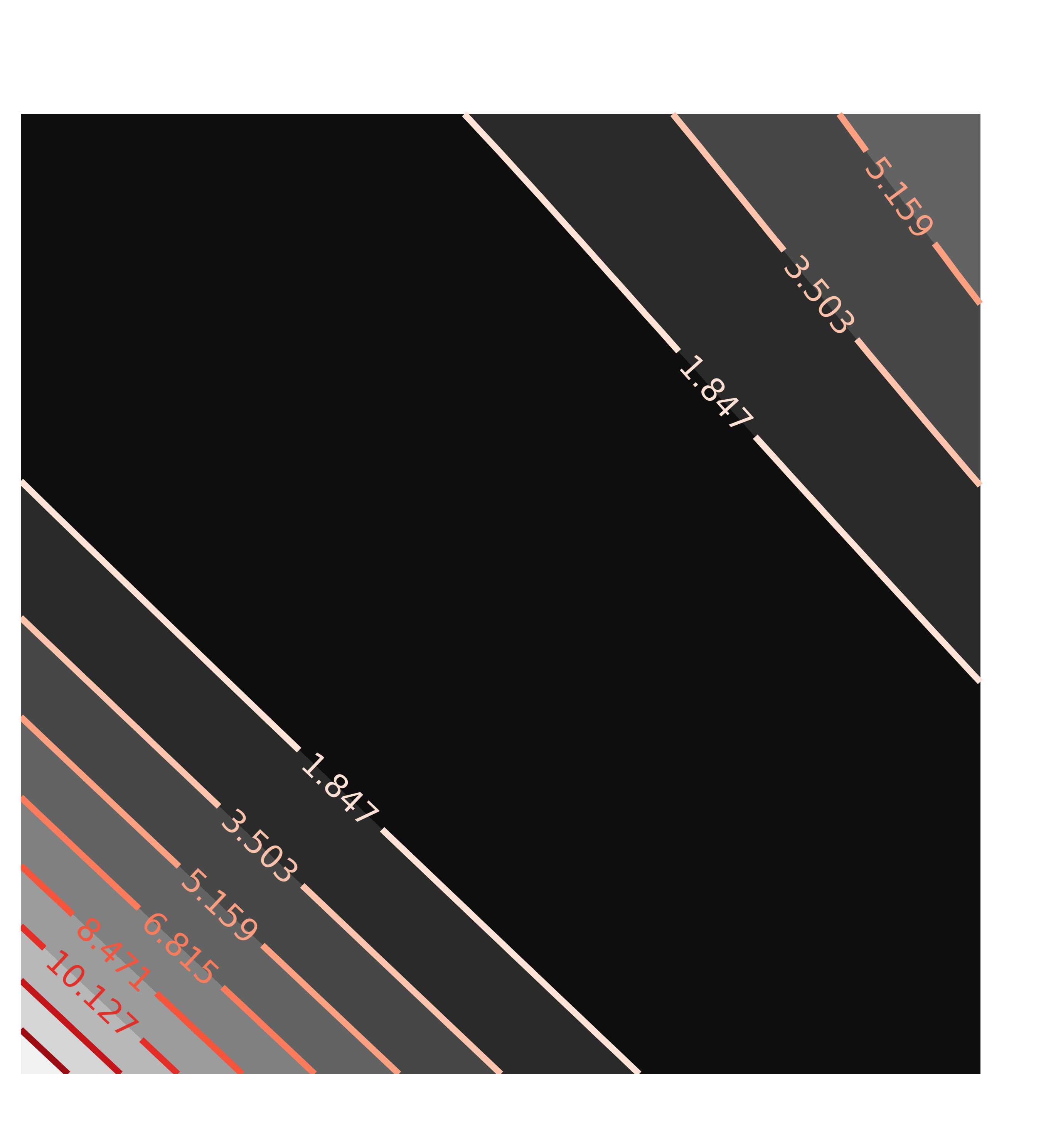
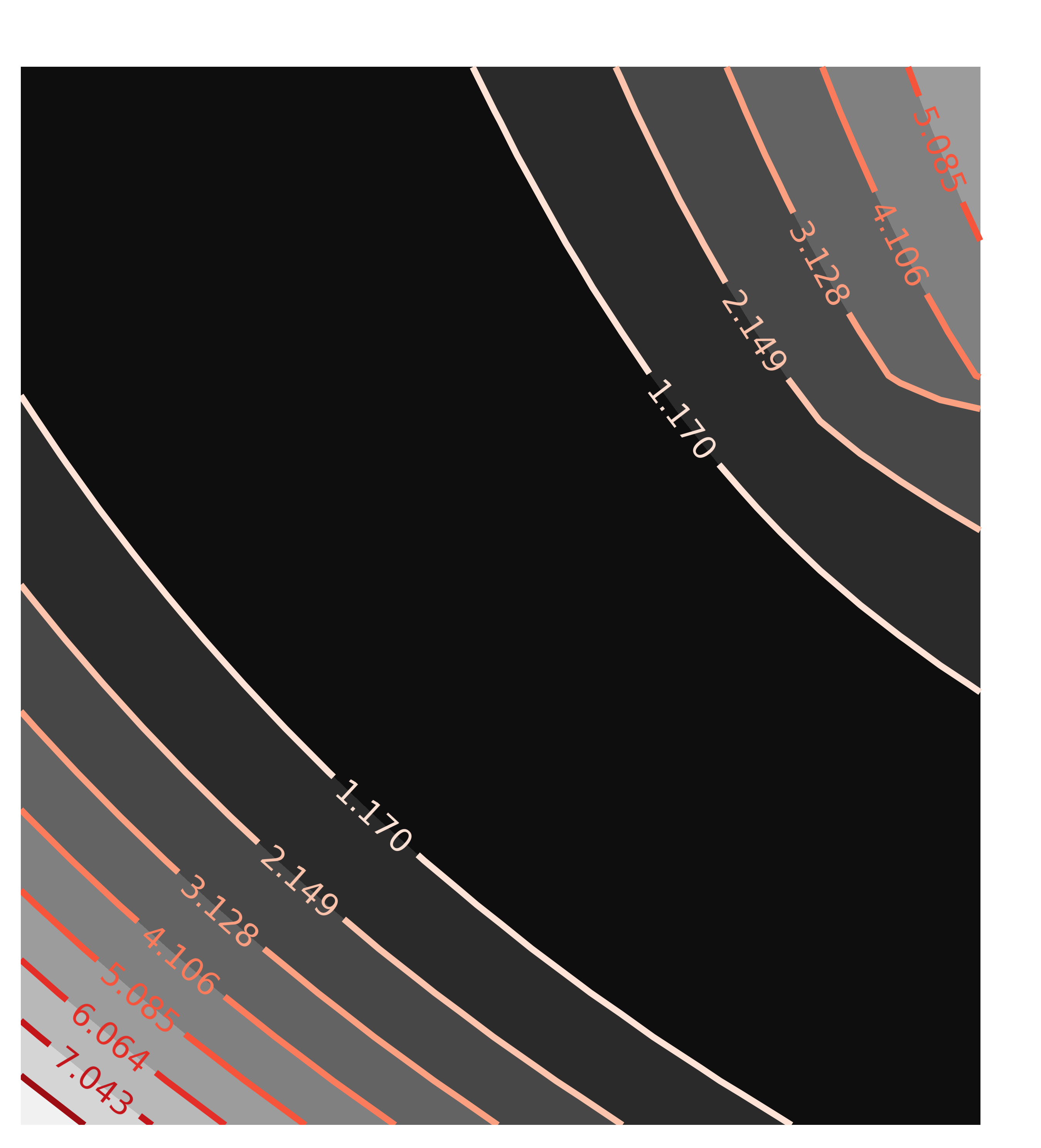
But now, if we turn to the more pathological case of the double exponential, we calculate the chi-square maps as:
x1, y1, c1 = chi2_map(minout, 'a1', 'a2', nx=25, ny=25)
x2, y2, c2 = chi2_map(minout, 'a1', 't1', nx=25, ny=25)
contour(c1, x=x1, y=y1,        title='Correlation(a1, a2)')
contour(c2, x=x2, y=y2, win=2, title='Correlation(a1, t1)')
with the resulting contour plots:
Here, the values of chi-square quickly grow very large away from the ideal fit. More importantly, the maps are not remotely elliptical.
Finally, it should be emphasized that while all the tests in this section are informative, they are also fairly slow, re-running the fits many times. It is probably safe to rely on the automatic calculations of uncertainties and correlations, and use these methods on occasions of extremely high correlation, or when nearing a final analysis.

