doc_model_composite.py

[[Model]]
    (Model(jump) <function convolve at 0x18205b600> Model(gaussian))
[[Fit Statistics]]
    # fitting method   = leastsq
    # function evals   = 33
    # data points      = 201
    # variables        = 3
    chi-square         = 24.7562335
    reduced chi-square = 0.12503148
    Akaike info crit   = -414.939746
    Bayesian info crit = -405.029832
    R-squared          = 0.99632577
[[Variables]]
    mid:        4 (fixed)
    amplitude:  0.62508458 +/- 0.00189732 (0.30%) (init = 1)
    center:     5.50853669 +/- 0.00973231 (0.18%) (init = 3.5)
    sigma:      0.59576097 +/- 0.01348579 (2.26%) (init = 1.5)
[[Correlations]] (unreported correlations are < 0.100)
    C(amplitude, center) = +0.3292
    C(amplitude, sigma)  = +0.2680

# <examples/doc_model_composite.py>
import matplotlib.pyplot as plt
import numpy as np

from lmfit import CompositeModel, Model
from lmfit.lineshapes import gaussian, step

# create data from broadened step
x = np.linspace(0, 10, 201)
y = step(x, amplitude=12.5, center=4.5, sigma=0.88, form='erf')
np.random.seed(0)
y = y + np.random.normal(scale=0.35, size=x.size)


def jump(x, mid):
    """Heaviside step function."""
    o = np.zeros(x.size)
    imid = max(np.where(x <= mid)[0])
    o[imid:] = 1.0
    return o


def convolve(arr, kernel):
    """Simple convolution of two arrays."""
    npts = min(arr.size, kernel.size)
    pad = np.ones(npts)
    tmp = np.concatenate((pad*arr[0], arr, pad*arr[-1]))
    out = np.convolve(tmp, kernel, mode='valid')
    noff = int((len(out) - npts) / 2)
    return out[noff:noff+npts]


# create Composite Model using the custom convolution operator
mod = CompositeModel(Model(jump), Model(gaussian), convolve)

# create parameters for model.  Note that 'mid' and 'center' will be highly
# correlated. Since 'mid' is used as an integer index, it will be very
# hard to fit, so we fix its value
pars = mod.make_params(amplitude=dict(value=1, min=0),
                       center=3.5,
                       sigma=dict(value=1.5, min=0),
                       mid=dict(value=4, vary=False))

# fit this model to data array y
result = mod.fit(y, params=pars, x=x)

print(result.fit_report())

# generate components
comps = result.eval_components(x=x)

# plot results
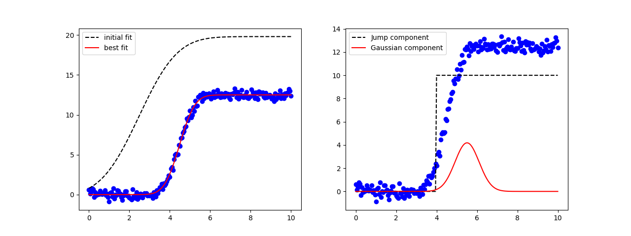
fig, axes = plt.subplots(1, 2, figsize=(12.8, 4.8))

axes[0].plot(x, y, 'bo')
axes[0].plot(x, result.init_fit, 'k--', label='initial fit')
axes[0].plot(x, result.best_fit, 'r-', label='best fit')
axes[0].legend()

axes[1].plot(x, y, 'bo')
axes[1].plot(x, 10*comps['jump'], 'k--', label='Jump component')
axes[1].plot(x, 10*comps['gaussian'], 'r-', label='Gaussian component')
axes[1].legend()

plt.show()
# <end examples/doc_model_composite.py>