9.6. XAFS: Wavelet Transforms for XAFS

Wavelet transforms extend Fourier transforms, effectively separating contributions of a waveform into both time and frequency (or, for EXAFS, \(k\) and \(R\)). A variety of mathematical kernels can be used for wavelet transforms. There are a few examples in the literature of applying wavelet transforms to EXAFS data, with the Cauchy wavelet used by Munoz et al [Larch_12] being one early application. The cauchy_wavelet() function described below follows this work, and that article should be cited as the reference for this transform.

9.6.1. cauchy_wavelet()

The Continuous Cauchy Wavelet transform of Munoz et al [Larch_12] is implemented as the function cauchy_wavelet():

_xafs.cauchy_wavelet(k, chi, group=None, kweight=0, rmax_out=10)

perform a Continuous Cauchy wavelet transform of \(\chi(k)\).

Parameters:

• k – 1-d array of photo-electron wavenumber in \(\rm\AA^{-1}\)
• chi – 1-d array of \(\chi\)
• group – output Group
• rmax_out – highest R for output data (10 \(\rm\AA\))
• kweight – exponent for weighting spectra by \(k^{\rm kweight}\)
• nfft – value to use for \(N_{\rm fft}\) (2048).

Returns:

None – outputs are written to supplied group.

If a group argument is provided of if the first argument is a Group, the following data arrays are put into it:

array name	meaning
r	uniform array of \(R\), out to rmax_out.
wcauchy	complex array cauchy transform of \(R\) and \(k\)
wcaychy_mag	magnitude of cauchy transform
wcauchy_re	real part of cauchy transform
wcauchy_im	imaginary part of cauchy transform

It is expected that the input k be a uniformly spaced array of values with spacing kstep, starting a 0.

9.6.2. Wavelet Example

Applying the Cauchy wavelet transform to Fe K-edge data of FeO is fairly straightforward:

# wavelet transform in larch
# follows method of Munuz, Argoul, and Farges

f = read_ascii('../xafsdata/feo_xafs.dat')
autobk(f, rbkg=0.9, kweight=2)

kopts = {'xlabel': r'$k \,(\AA^{-1})$', 
         'ylabel': r'$k^2\chi(k) \, (\AA^{-2})$', 
         'linewidth': 3, 'title': 'FeO', 'show_legend':True}

newplot(f.k, f.chi*f.k**2, win=1, label='original data', **kopts)

# do wavelet transform (no window function yet)
cauchy_wavelet(f, kweight=2)

# display wavelet magnitude, real part
# horizontal axis is k, vertical is R
imopts = {'x': f.k, 'y': f.r}
imshow(f.wcauchy_mag, win=1, label='Wavelet Transform: Magnitude', **imopts)
imshow(f.wcauchy_re,  win=2, label='Wavelet Transform: Real Part', **imopts)

# plot wavelet projected to k space
plot(f.k, f.wcauchy_re.sum(axis=0), win=1, label='projected wavelet', **kopts)

ropts = kopts
ropts['xlabel'] = r'$R \, (\AA) $'
ropts['ylabel'] = r'$|\chi(R)| \, (\AA^{-3})$'

# plot wavelet projected to R space
newplot(f.r, f.wcauchy_mag.sum(axis=1), win=2,  label='projected wavelet', **ropts)

With results for the Cauchy transforms looking like (here, \(k\)is along the horizontal axis extending to 16 \(\rm\AA^{-1}\), and with \(R\) along the vertical axis, increasing from 0 at the bottom to 10 \(\rm\AA\) at the top.

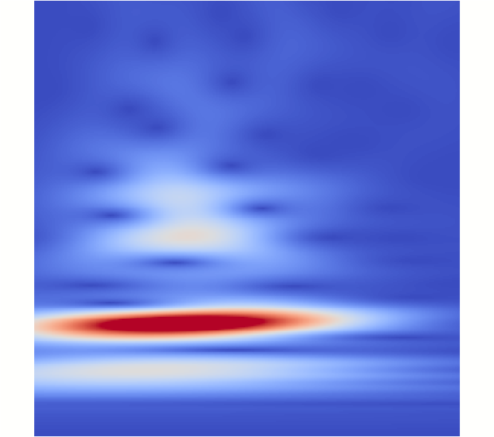
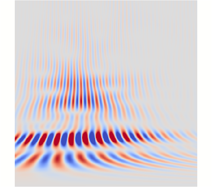
The Cauchy Wavelet transforms, with magnitude on the left hand panel and real part on the right hand panel.

The projection of the wavelets to \(k\) and \(R\) space looks like:

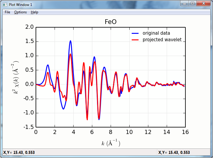
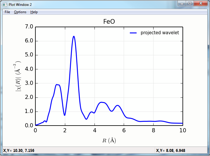
The Cauchy Wavelet transform projected to \(k\) and \(R\) space. In the left hand panel, the original EXAFS \(k^2\chi(k)\) is shown for comparison.

References

[Larch_12]

(1, 2) M. Munoz, P. Argoul, and F. Farges. Continuous Cauchy wavelet transform analyses of EXAFS spectra: A qualitative approach. American Mineralogist, 88(4):694–700, 2003.