$$

14.5. XAFS: Fourier Transforms for XAFS

Fourier transforms are central to understanding and using XAFS. Consequently, many of the XAFS functions in Larch use XAFS Fourier transforms as part of their processing, and many of the functions parameters and arguments described here have names and meanings used throughout the XAFS functionality of Larch. For example, both autobk() and feffit() rely on XAFS Fourier transforms, and use the XAFS Fourier transform function described here.

14.5.1. Overview of XAFS Fourier transforms

The standard Fourier transform of a signal $f(t)$ can be written as

$$\begin{array}{rcl}\tilde{f}(\omega )& =& \frac{1}{\sqrt{2\pi }}{\int }_{-\mathrm{\infty }}^{\mathrm{\infty }}f(t)e^{-i\omega t}dt\\ f(t)& =& \frac{1}{\sqrt{2\pi }}{\int }_{-\mathrm{\infty }}^{\mathrm{\infty }}\tilde{f}(\omega )e^{i\omega t}d\omega \end{array}$$

where the symmetric normalization is one of the more common choices of conventions. This gives conjugate variables of $\omega$ and $t$. Because XAFS goes as

$$\chi (k)\sim \sin [2kR+\delta (k)]$$

the conjugate variables in XAFS are generally taken to be $k$ and $2R$. The normalization of $\tilde{\chi }(R)$ from a Fourier transform of $\chi (k)$ is a matter of convention, but we follow the symmetric case above (with $t$ replaced by $k$ and $\omega$ replaced by $2R$, and of course $f$ by $\chi$).

But there are two more important issues to mention. First, an XAFS Fourier transform multiplies $\chi (k)$ by a power of $k$, $k^n$ and by a window function $\mathrm{\Omega }(k)$ before doing the Fourier transform. The power-law weighting allow the oscillations in $k$ to emphasize different portions of the spectra, or to give a uniform intensity to the oscillations. The window function acts to smooth the resulting Fourier transform and remove ripple and ringing in it that would result from a sudden truncation of $\chi (k)$ at the end of the data range.

The second important issue is that the continuous Fourier transform described above is replaced by a discrete transform. This better matches the discrete sampling of energy and $k$ values of the data, and allows Fast Fourier Transform techniques to be used. It does change the definitions of the transforms used somewhat. First, the $\chi (k)$ data must be on uniformly spaced set of $k$ values. The default $k$ spacing used in Larch (including as output from autobk()) is $\delta k$ = 0.05 ${\text{Å}}^{-1}$. Second, the array size for $\chi (k)$ used in the Fourier transform should be a power of 2. The default used in Larch is $N_{\mathrm{f}\mathrm{f}\mathrm{t}}$ = 2048. Together, these allow $\chi (k)$ data to 102.4 ${\text{Å}}^{-1}$. Of course, real data doesn’t extend that far, so the array to be transformed is zero-padded to the end of the range. Since the spacing $\delta R$ of the resulting discrete $\chi (R)$ is given as $\pi /(N_{\mathrm{f}\mathrm{f}\mathrm{t}}\delta k)$, the extended range and zero-padding will increase the density of points in $\chi (R)$, smoothly interpolating the values. For $N_{\mathrm{f}\mathrm{f}\mathrm{t}}$ = 2048 and $\delta k$ = 0.05 ${\text{Å}}^{-1}$, the $R$ spacing is approximately $\delta R$ = 0.0307 $\text{Å}$.

For the discrete Fourier transforms with samples of $\chi (k)$ at the points $k_n=n\delta k$, and samples of $\chi (R)$ at the points $R_m=m\delta R$, the definitions become:

$$\begin{array}{rcl}\tilde{\chi }(R_m)& =& \frac{i\delta k}{\sqrt{\pi N_{\mathrm{f}\mathrm{f}\mathrm{t}}}}\sum _{n=1}^{N_{\mathrm{f}\mathrm{f}\mathrm{t}}}\chi (k_n)\mathrm{\Omega }(k_n)k_n^w{e}^{2i\pi nm/N_{\mathrm{f}\mathrm{f}\mathrm{t}}}\\ \tilde{\chi }(k_n)& =& \frac{2i\delta R}{\sqrt{\pi N_{\mathrm{f}\mathrm{f}\mathrm{t}}}}\sum _{m=1}^{N_{\mathrm{f}\mathrm{f}\mathrm{t}}}\tilde{\chi }(R_m)\mathrm{\Omega }(R_m)e^{-2i\pi nm/N_{\mathrm{f}\mathrm{f}\mathrm{t}}}\end{array}$$

These normalizations preserve the symmetry properties of the Fourier Transforms with conjugate variables $k$ and $2R$. Though the reverse transform converts the complex $\chi (R)$ to the complex $\chi (k)$ on the same $k$ spacing as the starting data, we often refer to the filtered $\chi (k)$ as q space.

A final complication in using Fourier transforms for XAFS is that the measured $\mu (E)$ and $\chi (k)$ are a strictly real values, while the Fourier transform inherently treats $\chi (k)$ and $\chi (R)$ as complex values. This leads to an ambiguity about how to construct the complex $\tilde{\chi }(k)$. In many formal treatments, XAFS is written as the imaginary part of a complex function. This might lead one to assume that constructing $\tilde{\chi }(k)$ as $0+i\chi (k)$ would be the natural choice. For historical reasons, Larch uses the opposite convention, constructing $\tilde{\chi }(k)$ as $\chi (k)+0i$. As we’ll see below, you can easily change this convention. The effect of this choice is minor unless one is concerned about the differences of the real and imaginary parts of $\chi (R)$ or one is intending to filter and back-transform the $\chi (R)$ and compare the filtered and unfiltered data.

14.5.2. Forward XAFS Fourier transforms ($k\to R$)

The forward Fourier transform converts $\chi (k)$ to $\chi (R)$ and is of primary importance for XAFS analysis. In Larch, this is encapsulated in the xftf() function.

xftf(k, chi=None, group=None, ...)

perform a forward XAFS Fourier transform, from $\chi (k)$ to $\chi (R)$, using common XAFS conventions.

Parameters:

• k – 1-d array of photo-electron wavenumber in ${\text{Å}}^{-1}$

• chi – 1-d array of $\chi$

• group – output Group

• rmax_out – highest R for output data (10 $\text{Å}$)

• kweight – exponent for weighting spectra by $k^{\mathrm{k}\mathrm{w}\mathrm{e}\mathrm{i}\mathrm{g}\mathrm{h}\mathrm{t}}$

• kmin – starting k for FT Window

• kmax – ending k for FT Window

• dk – tapering parameter for FT Window

• dk2 – second tapering parameter for FT Window

• window – name of window type

• nfft – value to use for $N_{\mathrm{f}\mathrm{f}\mathrm{t}}$ (2048).

• kstep – value to use for $\delta k$ (0.05).

Returns:

None – outputs are written to supplied group.

Follows the First Argument Group convention, using group members named k and chi. The following data is put into the output group:

array name	meaning
kwin	window $\mathrm{\Omega }(k)$ (length of input chi(k)).
r	uniform array of $R$, out to rmax_out.
chir	complex array of $\tilde{\chi }(R)$.
chir_mag	magnitude of $\tilde{\chi }(R)$.
chir_pha	phase of $\tilde{\chi }(R)$.
chir_re	real part of $\tilde{\chi }(R)$.
chir_im	imaginary part of $\tilde{\chi }(R)$.

It is expected that the input k be a uniformly spaced array of values with spacing kstep, starting a 0. If it is not, the k and chi data will be linearly interpolated onto the proper grid.

The FT window parameters are explained in more detail in the discussion of ftwindow().

xftf_fast(chi, nfft=2048, kstep=0.05)

perform a forward XAFS Fourier transform, from $\chi (k)$ to $\chi (R)$, using common XAFS conventions. This version demands chi to include any weighting and windowing, and so to represent $\chi (k)k^w\mathrm{\Omega }(k)$ on a uniform $k$ grid. It returns the complex array of $\chi (R)$.

Parameters:

• chi – 1-d array of $\chi$ to be transformed

• nfft – value to use for $N_{\mathrm{f}\mathrm{f}\mathrm{t}}$ (2048).

• kstep – value to use for $\delta k$ (0.05).

Returns:

complex $\chi (R)$.

14.5.3. Reverse XAFS Fourier transforms ($R\to q$)

Reverse Fourier transforms convert $\chi (R)$ back to filtered $\chi (k)$. We refer to the filtered $k$ space as $q$ to emphasize the distinction between the two. The filtered $\chi (q)$ is complex. By convention, the real part of $\chi (q)$ corresponds to the explicitly real $\chi (k)$.

xftr(r, chir, group=None, ...)

perform a reverse XAFS Fourier transform, from $\chi (R)$ to $\chi (q)$.

Parameters:

• r – 1-d array of distance.

• chir – 1-d array of $\chi (R)$

• group – output Group

• qmax_out – highest k for output data (30 ${\text{Å}}^{-1}$)

• rweight – exponent for weighting spectra by $r^{\mathrm{r}\mathrm{w}\mathrm{e}\mathrm{i}\mathrm{g}\mathrm{h}\mathrm{t}}$ (0)

• rmin – starting R for FT Window

• rmax – ending R for FT Window

• dr – tapering parameter for FT Window

• dr2 – second tapering parameter for FT Window

• window – name of window type

• nfft – value to use for $N_{\mathrm{f}\mathrm{f}\mathrm{t}}$ (2048).

• kstep – value to use for $\delta k$ (0.05).

Returns:

None – outputs are written to supplied group.

Follows the First Argument Group convention, using group members named r and chir. The following data is put into the output group:

array name	meaning
rwin	window $\mathrm{\Omega }(R)$ (length of input chi(R)).
q	uniform array of $k$, out to qmax_out.
chiq	complex array of $\tilde{\chi }(k)$.
chiq_mag	magnitude of $\tilde{\chi }(k)$.
chiq_pha	phase of $\tilde{\chi }(k)$.
chiq_re	real part of $\tilde{\chi }(k)$.
chiq_im	imaginary part of $\tilde{\chi }(k)$.

In analogy with xftf(), it is expected that the input r be a uniformly spaced array of values starting a 0.

The input chir array can be either the complex $\chi (R)$ array as output to Group.chir from xftf(), or one of the real or imaginary parts of the $\chi (R)$ as output to Group.chir_re or Group.chir_im.

The FT window parameters are explained in more detail in the discussion of ftwindow().

xftr_fast(chir, nfft=2048, kstep=0.05)

perform a reverse XAFS Fourier transform, from $\chi (R)$ to $\chi (q)$, using common XAFS conventions. This version demands chir be the complex $\chi (R)$ as created from xftf(). It returns the complex array of $\chi (q)$ without putting any values into a group.

Parameters:

• chir – 1-d array of $\chi (R)$ to be transformed

• nfft – value to use for $N_{\mathrm{f}\mathrm{f}\mathrm{t}}$ (2048).

• kstep – value to use for $\delta k$ (0.05).

Returns:

complex $\chi (q)$.

14.5.4. ftwindow(): Generating Fourier transform windows

As mentioned above, a Fourier transform window will smooth the resulting Fourier transformed spectrum, removing ripple and ringing in it that would result from a sudden truncation data at the end of it range. There is an extensive literature on such windows, and a lot of choices and parameters available for constructing windows. A sampling of windows is shown below.

ftwindow(x, xmin=0, xmax=None, dk=1, ...)

create a Fourier transform window array.

Parameters:

• x – 1-d array array to build window on.

• xmin – starting x for FT Window

• xmax – ending x for FT Window

• dx – tapering parameter for FT Window

• dx2 – second tapering parameter for FT Window (=dx)

• window – name of window type

Returns:

1-d window array.

Note that if dx is specified but dx2 is not, dx2 will generally take the same value as dx.

The window type must be one of those listed in the Table of Fourier Transform Window Types.

Table of Fourier Transform Window Types.

window name	description
hanning	cosine-squared taper
parzen	linear taper
welch	quadratic taper
gaussian	Gaussian (normal) function window
sine	sine function window
kaiser	Kaiser-Bessel function-derived window

In general, the window arrays have a value that gradually increases from 0 up to 1 at the low-k end, may stay with a value 1 over some central portion, and then tapers down to 0 at the high-k end. The meaning of the dx and dx2, and even xmin, and xmax varies a bit for the different window types. The Hanning, Parzen, and Welch windows share a convention that the windows taper up from 0 to 1 between xmin-dx/2 and xmin+dx/2, and then taper down from 1 to 0 between xmax-dx2/2 and xmax+dx2/2.

The conventions for the Kaiser, Gaussian, and Sine window types is a bit more complicated, and is best given explicitly. In the formulas below, dx written as $dx$ and dx2 as $d{x}_2$. We define $x_i=x_{\mathrm{m}\mathrm{i}\mathrm{n}}-dx/2$, $x_f=x_{\mathrm{m}\mathrm{a}\mathrm{x}}+d{x}_2/2$, and $x_0=(x_f+x_i)/2$, as the beginning, end, and center of the widows. For the Gaussian window, the form is:

$$\mathrm{\Omega }(x)=\exp [-\frac{(x-x_0{)}^2}{2{dx}^2}]$$

The form for the Sine window is

$$\mathrm{\Omega }(x)=\sin [\frac{\pi (x_f-x)}{x_f-x_i}]$$

between $x_i$ and $x_f$, and 0 outside this range. The Kaiser-Bessel window is slightly more complicated:

$$\begin{array}{rcl}a& =& \sqrt{max[0,1-\frac{4(x-x_0{)}^2}{(x_f-x_i{)}^2}]}\\ \mathrm{\Omega }(x)& =& \frac{i_0(adx)-1}{i_0(dx)-1}\end{array}$$

where $i_0$ is the modified Bessel function of order 0.

14.5.5. Catalog of Fourier transform window

Here, we give a series of example windows, to illustrate the different window types and the effect of the various parameters. The meanings of xmin, xmax, dx and dx2 are identical for the Hanning, Parzen and Welch windows, and illustrated in the two following figures.

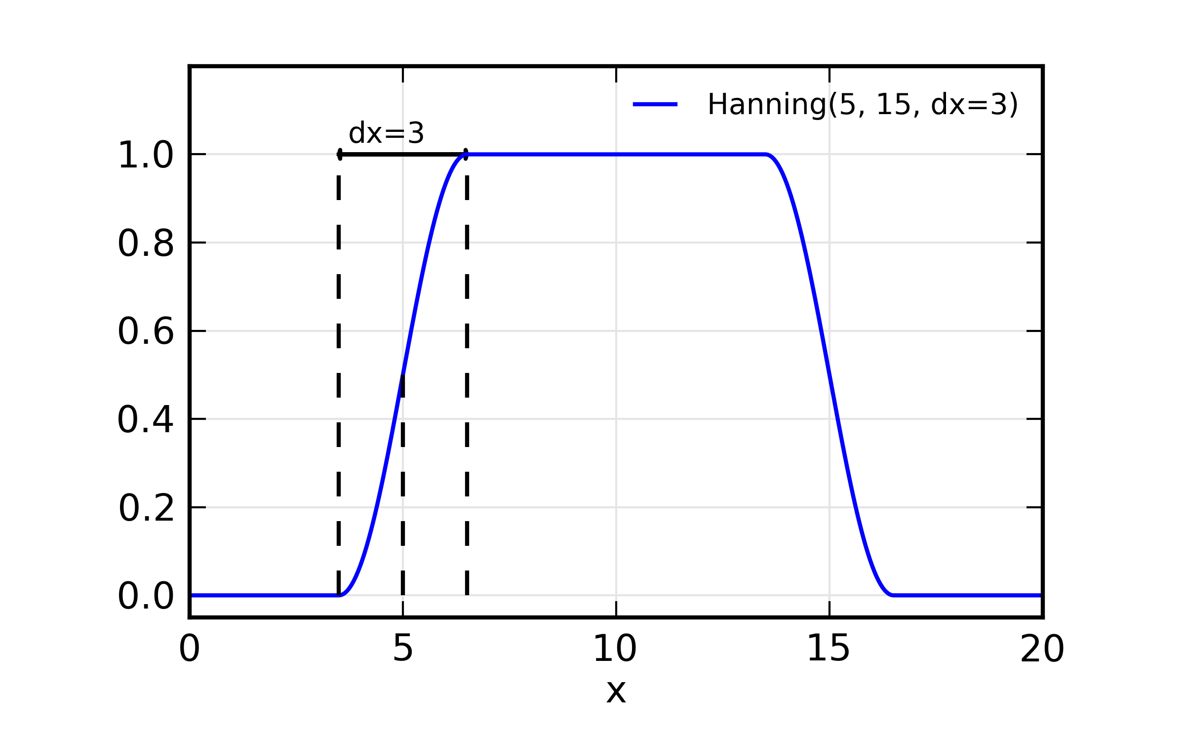
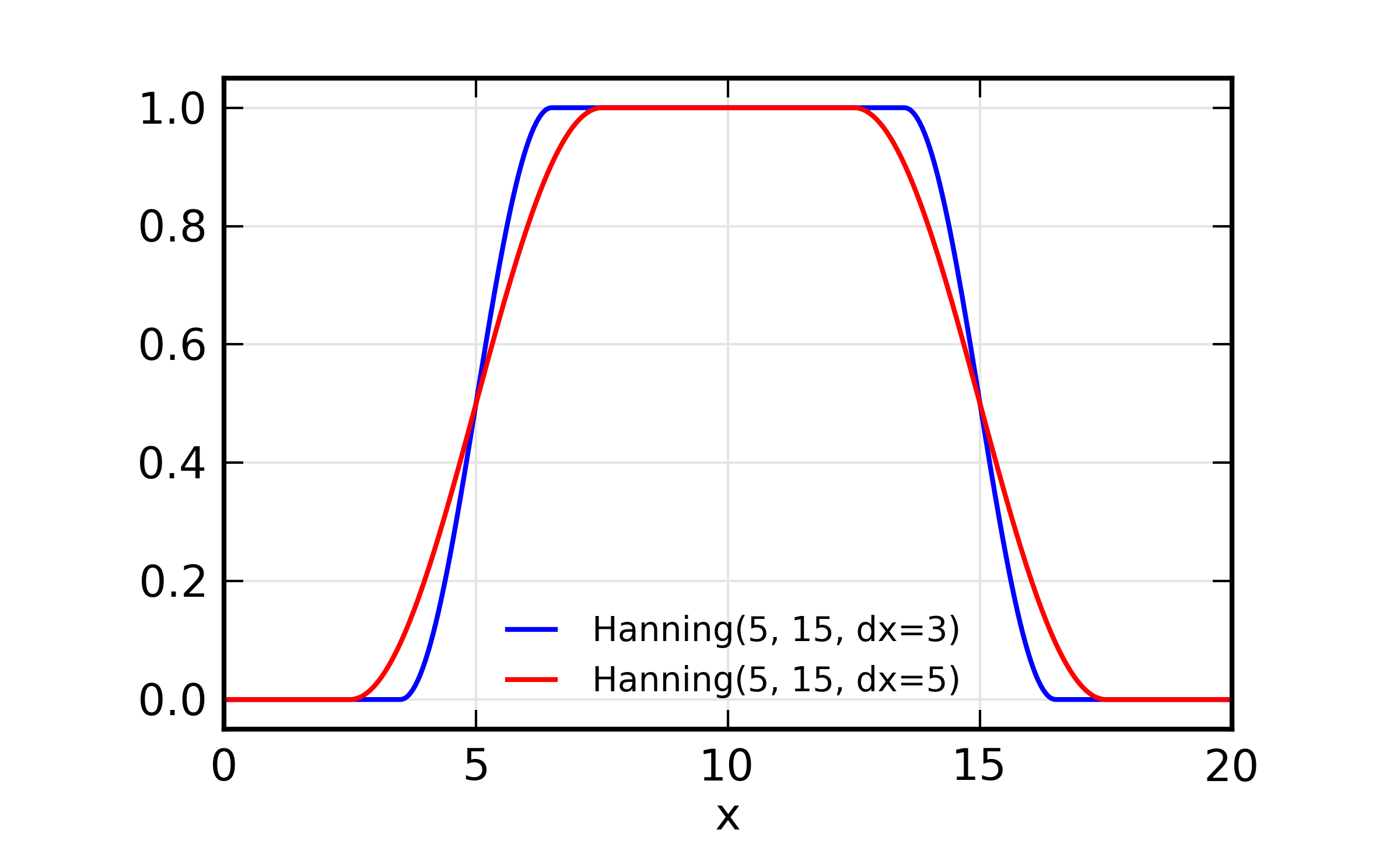
Fourier Transform window examples and illustration of parameter meaning for the Hanning, Parzen, and Welch windows. Note that $\mathrm{\Omega }(x=x_{\mathrm{m}\mathrm{i}\mathrm{n}})=\mathrm{\Omega }(x=x_{\mathrm{m}\mathrm{a}\mathrm{x}})=0.5$, and that the meaning of dx is to control the taper over which the window changes from 0 to 1. Here, xmin=5 and xmax=15.

Some more window functions:

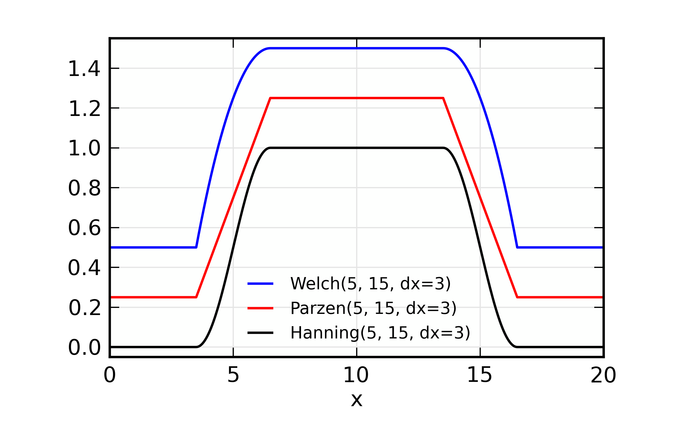
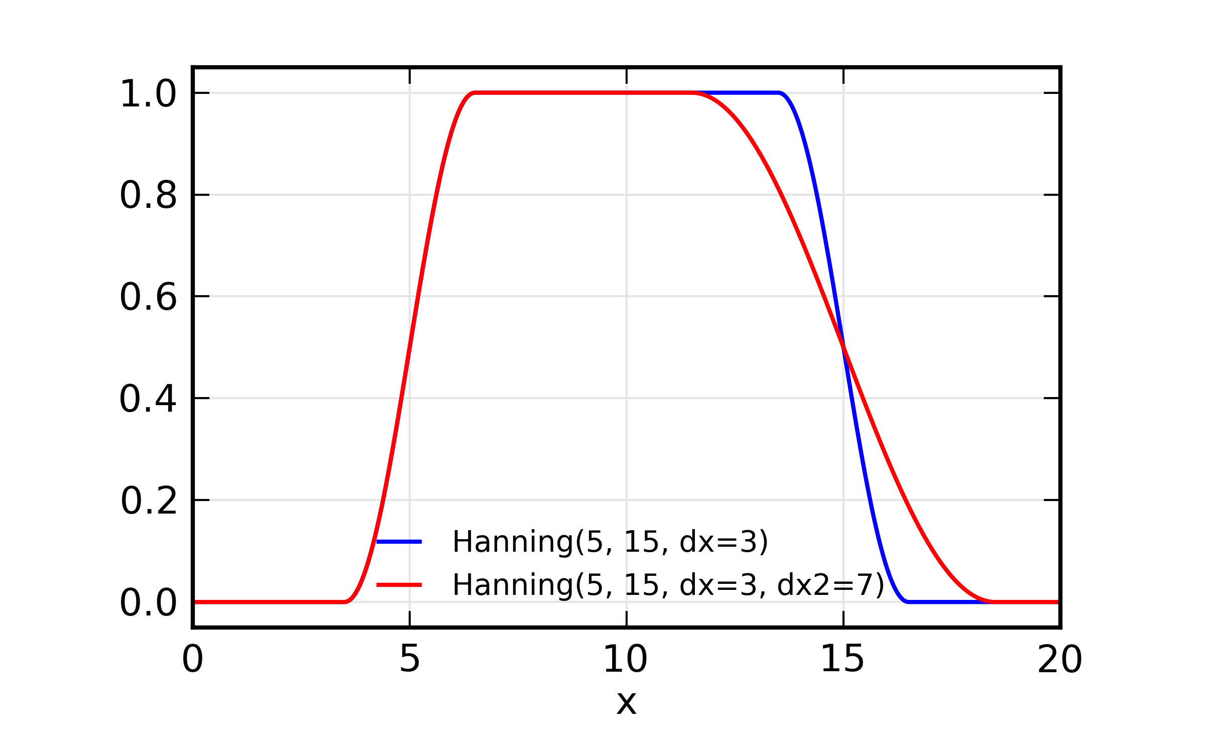
Fourier Transform window examples and illustration of parameter meaning. On the left, a comparison of Welch, Parzen, and Hanning with the same parameters is shown. On the right, the effect of dx2 is shown as a different amount of taper on the high- and low-x end of the window. As before, xmin=5 and xmax=15.

The Gaussian, Sine, and Kaiser-Bessel windows are illustrated next. These go to 1 at the average of xmin and xmax, but do not stay at 1 over a central portion of the window – they taper continuously. The Gaussian window is a simple Gaussian function, and is not truncated according to xmin and xmax, and the dx parameter sets the width. The Sine and Kaiser-Bessel windows both go to zero at xmin-dx/2 and xmax + dx/2. For very large values of dx, the Kaiser-Bessel window approaches a nearly Gaussian lineshape.

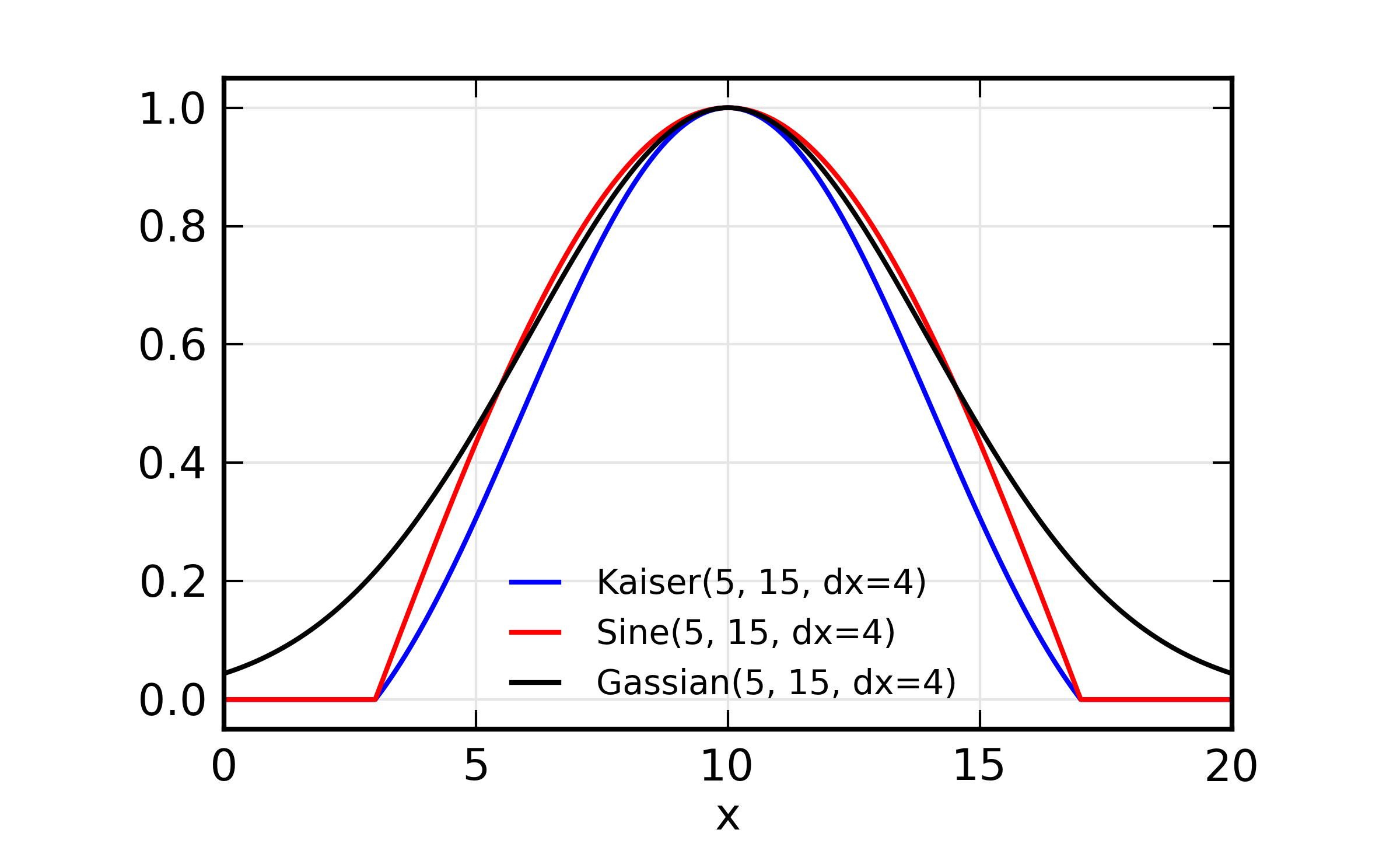
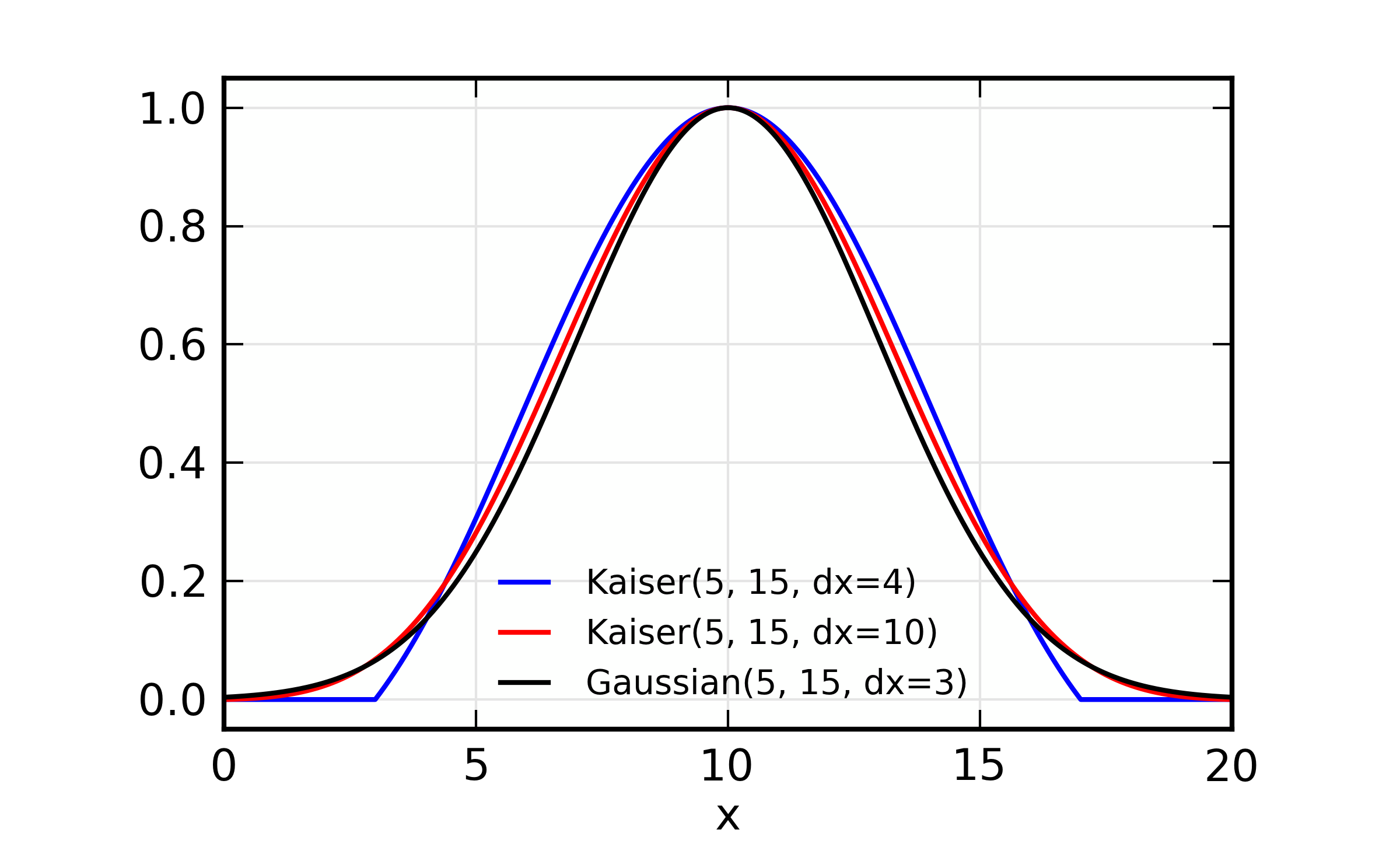
Fourier Transform windows. On the left, a comparison of Kaiser-Bessel, Sine, and Gaussian windows with the same parameters is shown. On the right, the effect of dx is shown for the Kaiser-Bessel window, and a closer comparison to a Gaussian window is made.

14.5.6. Examples: Forward XAFS Fourier transforms

Now we show some example Fourier transforms, illustrating the real and imaginary parts of the $\chi (R)$ as well as the magnitude, the effect of different windows types, and Fourier filtering to $\chi (q)$. We use a single XAFS dataset from FeO for all these examples, with a well-separated first and second shell. The full scripts to generate the figures shown here are included in the examples/xafs/ folder.

We start with a comparison of a small value of dk and a larger value. A script that runs xftf(), changing on dk would look like:

xftf(dat1.k, dat1.chi, kmin=3, kmax=13, dk=1, window='hanning',
     kweight=kweight, group=dat1)

dat2 = group(k=dat1.k, chi=dat1.chi) # make a copy of the group
xftf(dat2.k, dat2.chi, kmin=3, kmax=13, dk=5, window='hanning',
     kweight=kweight, group=dat2)

would result in the following results:

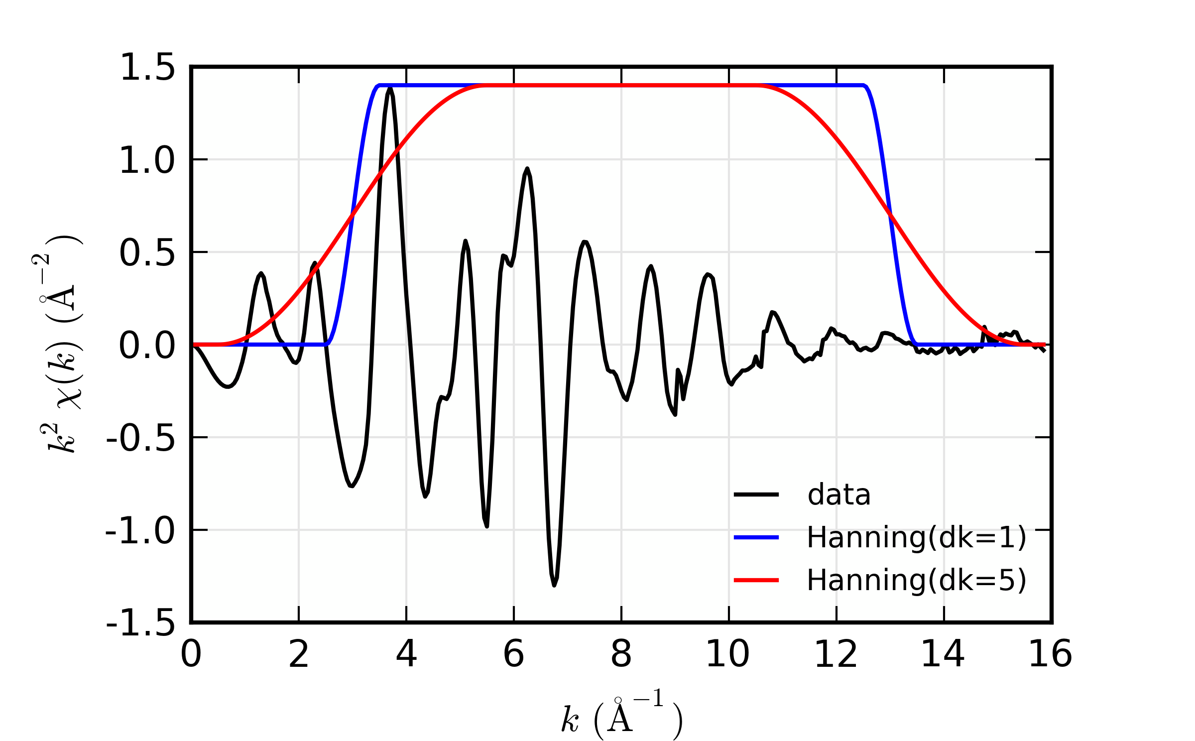
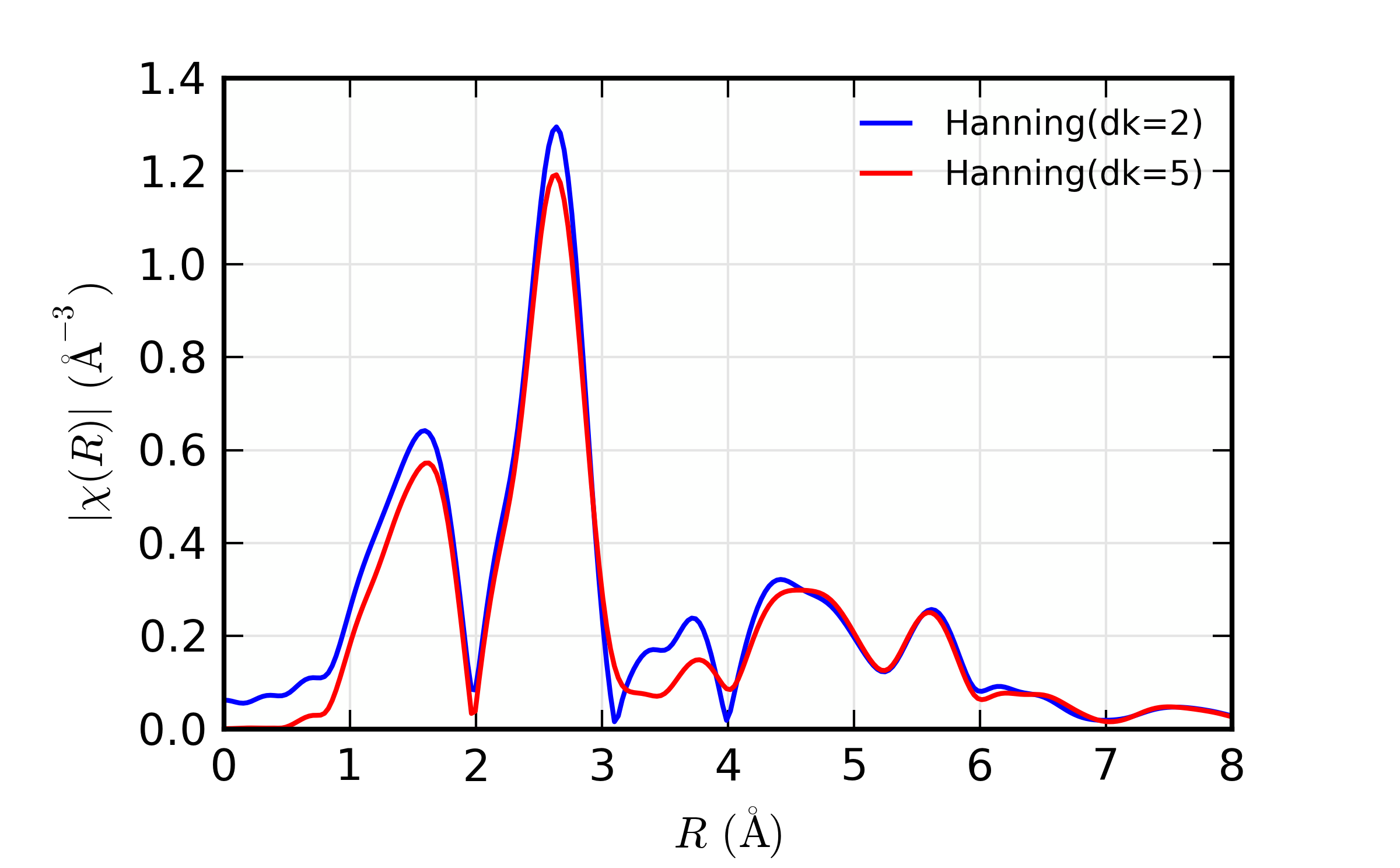
Comparison of the effect of different values of dk on real XAFS Fourier transforms. Increasing dk reduces peak heights and tends to broaden peaks, but the effects are rather small.

A script that runs xftf() with consistent parameters, but different window types:

xftf(dat1.k, dat1.chi, kmin=3, kmax=13, dk=4, window='hanning',
     kweight=kweight, group=dat1)

dat2 = group(k=dat1.k, chi=dat1.chi) # make a copy of the group
xftf(dat2.k, dat2.chi, kmin=3, kmax=13, dk=4, window='parzen',
     kweight=kweight, group=dat2)

dat3 = group(k=dat1.k, chi=dat1.chi) #
xftf(dat3.k, dat3.chi, kmin=3, kmax=13, dk=4, window='welch',
     kweight=kweight, group=dat3)

dat4 = group(k=dat1.k, chi=dat1.chi) #
xftf(dat4.k, dat4.chi, kmin=3, kmax=13, dk=4, window='kaiser',
     kweight=kweight, group=dat4)

dat5 = group(k=dat1.k, chi=dat1.chi) #
xftf(dat5.k, dat5.chi, kmin=3, kmax=13, dk=4, window='gaussian',
     kweight=kweight, group=dat5)

would result in the following results:

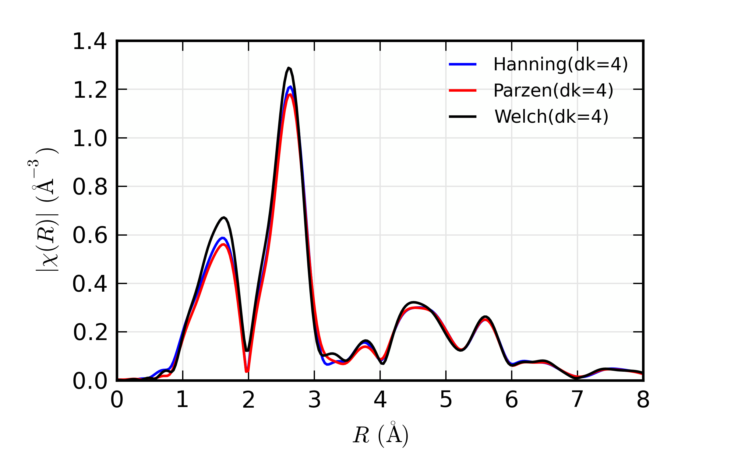
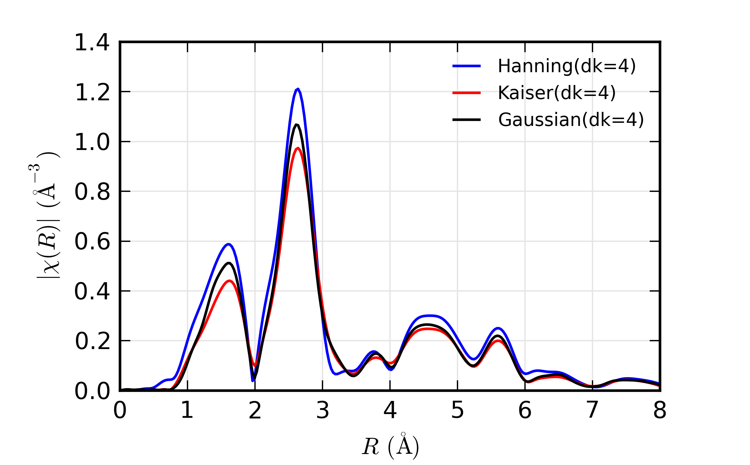
Comparison of the effect of different window types on real XAFS Fourier transforms.

We now turn our attention to the different components of the Fourier transform. As above, it is most common to plot the magnitude of the Fourier transform. But, as the transformed $\chi (R)$ is complex, it can be instructive to plot the real and imaginary components, as shown below:

newplot(dat1.r, dat1.chir_mag, xmax=8, label='chir_mag',
        show_legend=True, legend_loc='ur', color='black',
        xlabel=r'$R \rm\, (\AA)$', ylabel=r'$\chi(R)\rm\,(\AA^{-3})$' )

plot(dat1.r, dat1.chir_re, color='red', label='chir_re')
plot(dat1.r, dat1.chir_im, color='blue', label='chir_im')

which results in

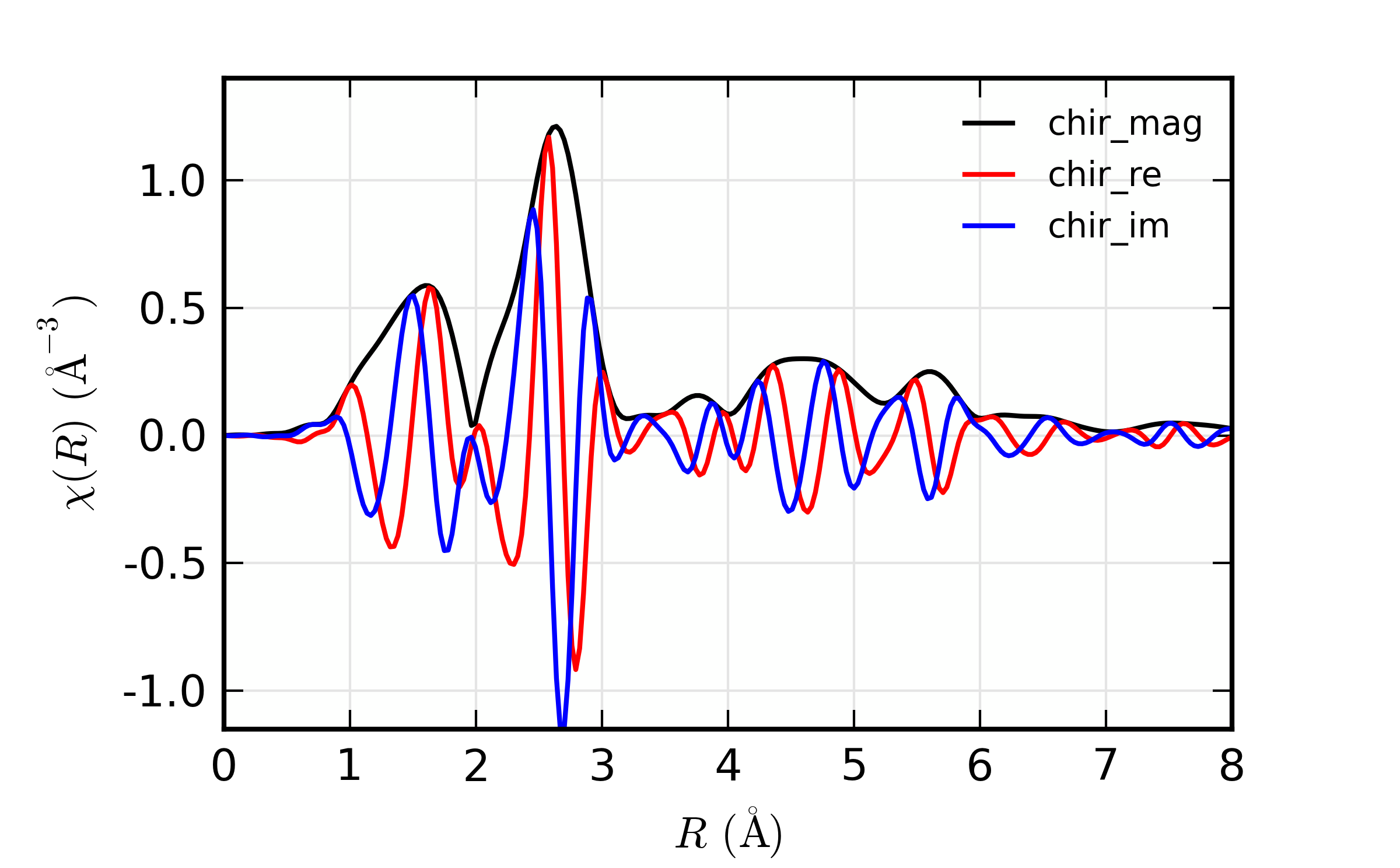
Figure 14.5.6.1 The real and imaginary components of the XAFS Fourier transform.

In fact, in the analysis discussed with feffit(), the real and imaginary components are used, not simply the magnitude.

14.5.7. Examples: Reverse XAFS Fourier transforms, Fourier Filtering

A reverse Fourier transform will convert data from $\chi (R)$ to $\chi (q)$. This allows a limited range of frequencies (distances) to be isolated and turned back into a $\chi (k)$ spectrum. Here, we show two different $R$ windows to filter either just the first shell of the spectra, or the first two shells, and compare the resulting filtered $\chi (q)$.

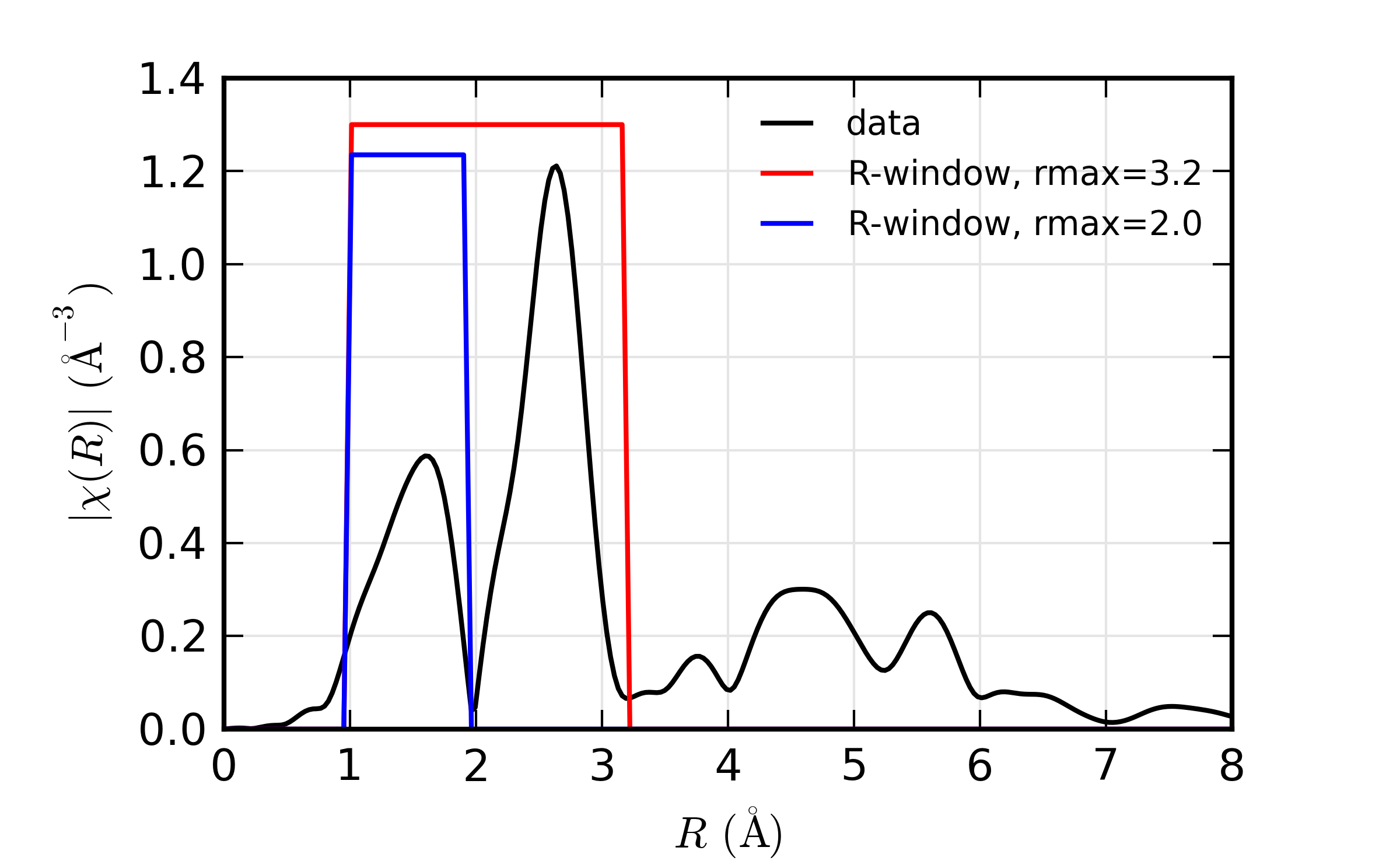
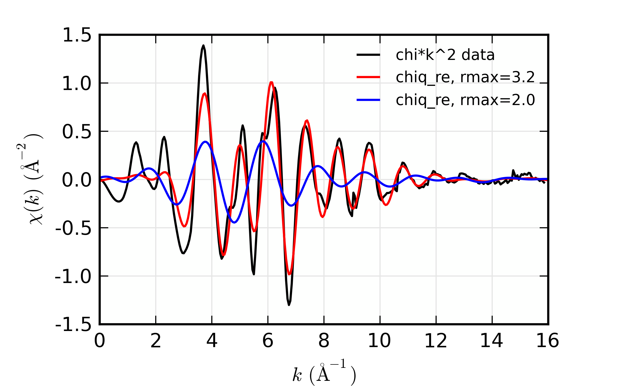
Reverse XAFS Fourier transform, or Fourier filtering. Here, one can see the effect of different window sizes on the Fourier filtered spectrum. Including the first two peaks or shells reproduces most of the original spectrum, with only high-frequency components removed.

Note that it is chiq_re that is compared to the k-weighted chi array.