
14.9. XAFS: Computing anomalous scattering factors from XAFS data
An input XAFS spectra is used to generate energy-dependent, anomalous scattering factors. This is used to improve upon the bare atom anomalous scattering factors of [Cromer and Liberman (1981)], [Chanter (2000)], and others near the absorption edge.
Since XAFS is sensitive to the atomic environment of the resonant atom (through the variations of the absorption coefficient), the scattering factors from the differential KK transform will also be sensitive to the local atomic structure of the resonant atom. These scattering factors, which are sensitive to chemical state and atomic environment, may be useful for many x-ray scattering and imaging experiments near resonances. The primary application is for the interpretation of fixed-q absorption experiments, such diffraction anomalous fine-structure (DAFS) or reflectively-EXAFS (sometimes known as ReflEXAFS).
14.9.1. Overview of the diffKK implementation
This performs the same algorithm as the venerable DIFFKK program described in [Cross et al. (1998)]. This uses the MacLaurin series algorithm to compute the differential (i.e. difference between the data and the tabulated \(f''(E)\)) Kramers-Kronig transform. This algorithm is described in [Ohta and Ishida (1988)]. This implementation casts the MacLaurin series algorithm in vectorized form using NumPy, so it is reasonably fast – not quite as fast as the original Fortran diffKK program, but certainly speedy enough for interactive data processing.
The input \(\mu(E)\) data are first matched to the tabulated \(f''(E)\) using the MBACK algorithm of [Weng, Waldo, and Penner-Hahn (2005)] with an option of using the modification proposed by [Lee et al. (2009)]. This scales the measured \(\mu(E)\) to the size of the tabulated function and adjusts the overall slope of the data to best match the tabulated value. This is seen at the top of Figure Figure 14.9.1.1.
The difference between the scaled \(\mu(E)\) and the tabulated \(f''(E)\) is then subjected to the KK transform. The result is added to the tabulated \(f'(E)\) spectrum to produce the resulting real part of the energy-dependent complex scattering factor. This is shown at the bottom of Figure 14.9.1.1.
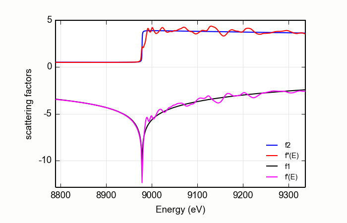
Figure 14.9.1.1 The anomalous scattering factors determined for copper metal from a copper foil, compared with the bare-atom, Cromer-Liberman values.
- diffkk(energy=None, mu=None, z=None, edge='K', mback_kws=None)
create a diffKK Group.
- Parameters:
energy – an array containing the energy axis of the measurement
mu – an array containing the measured \(\mu(E)\)
z – the Z number of the absorber element
edge – the edge measured, usually K or L3
mback_kws – arguments passed to the MBACK algorithm
- Returns:
a diffKK Group.
- diffkk.kk(energy=None, mu=None, z=None, edge='K', mback_kws=None)
Perform the KK transform.
- Parameters:
energy – an array containing the energy axis of the measurement
mu – an array containing the measured \(\mu(E)\)
z – the Z number of the absorber element
edge – the edge measured, usually K or L3
mback_kws – arguments passed to the MBACK algorithm
- Returns:
None
The following data is put into the diffKK group:
attribute
meaning
f2
array of tabulated \(f''(E)\)
f1
array of tabulated \(f'(E)\)
fpp
array of normalized \(f''(E)\)
fp
array of KK transformed \(f'(E)\)
All four arrays are on the same energy grid as the input data.
Here is an example script to make the figure shown above:
print 'Reading copper foil data'
data=read_ascii('../xafsdata/cu_10k.xmu')
dkk=diffkk(data.energy, data.mu, z=29, edge='K', mback_kws={'e0':8979, 'order':4})

print 'Doing diff KK transform'
dkk.kk()

newplot(dkk.energy, dkk.f2, label='f2', xlabel='Energy (eV)', ylabel='scattering factors',
        show_legend=True, legend_loc='lr')
plot(dkk.energy, dkk.fpp, label='f"(E)')
plot(dkk.energy, dkk.f1,  label='f1')
plot(dkk.energy, dkk.fp,  label='f\'(E)')
14.9.2. diffKK on L edge data
The diffKK method is fairly straightforward for K edge data. The algorithm for matching the measured \(\mu(E)\) to the tabulated \(f''(E)\) works quite well over the entire data range, resulting in a relatively unambiguous determination of \(f'(E)\). The situation for L edge data is a bit more complicated.
Consider the CeO2L edge data shown on the right on Figure 14.9.2.1. For these data, the matching algorithm is quite a bit more challenging, in part due to the very large spectral weight underneath the white lines and in part because the step size ratios in real data may not match the step size ratios in the tabulated \(f'(E)\).
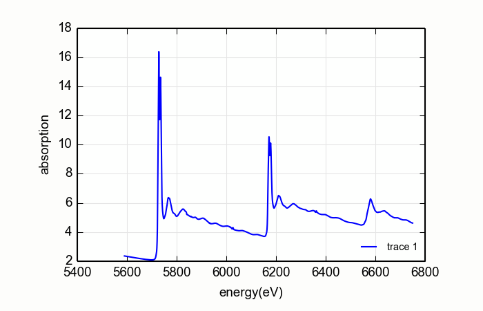 L-edge data
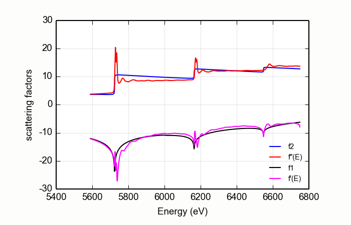 poor diffKK result
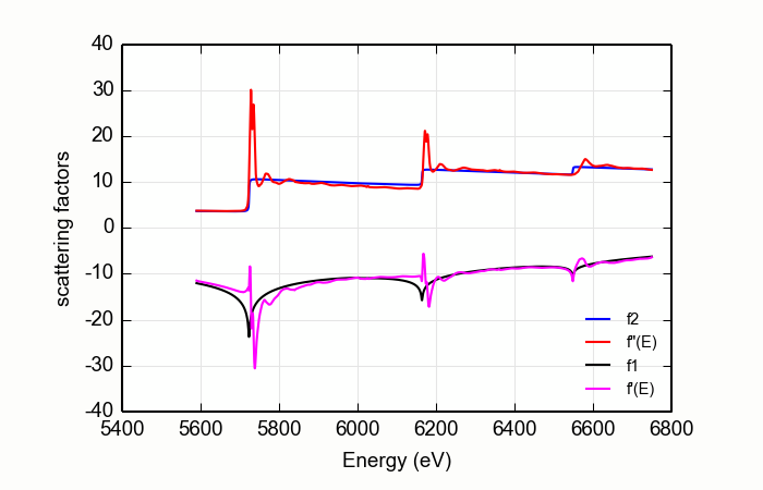 better diffKK result
Figure 14.9.2.1 DiffKK analysis of CeO2 L edge data
These larch command created the center plot in Figure 14.9.2.1.
data=read_ascii('CeO2_L321.xmu')
dkk=diffkk(data.e, data.xmu, z=58, edge='L3', mback_kws={'e0':5723, 'order':2})
dkk.kk()
The large white lines of the L3and L2edges cause an upwards slope in the function used to match the measured data to the tabulated data. This results in a suspicious \(f'(E)\). The situation is even worse when a higher order polynomial is used for the normalization.
The situation is improved somewhat by a simple trick.
data=read_ascii('CeO2_L321.xmu')
dkk=diffkk(data.e, data.xmu, z=58, edge='L3', mback_kws={'e0':5723, 'order':2, 'whiteline':20})
dkk.kk()
The result is shown in Figure 14.9.2.1. A margin is placed around the L3and L2white lines. The data from the white line energies to 20 eV above are excluded when determining the matching parameters. This does a somewhat nicer job of forcing the flat parts of measured data to match the tabulated data.
This seems to do a decent job of producing the \(f'(E)\) data. Still, this exposes a shortcoming of the diffKK algorithm for L edge data. This might be addressed by calculations of bare-atom scattering factors that better estimate the step ratios of real material. Another possibility is measurement of data over much longer data ranges so that the matching algorithm can be made to do a good job far away from the absorption edges. Or perhaps a non-differential algorithm would be more appropriate for L edge data.