Interactive wxmplot displays

The wxmplot Overview describes the main features of wxmplot and shows how wxmplot plotting functions give a richer level of customization and interactivity to the end user than is available from the standard matplotlib.pyplot. Here, the emphasis is on the immediacy of the interactivity of the data displays especially when used from interactive sessions. An important feature of the plot(), imshow() and other functions of the interactive module is that they display their results immediately, without having to execute a show() method to render the display. For interactive work from the Python (or one of the Jupyter consoles or notebook) prompt, the displayed windows do not block the Python session. This means that not only can you zoom in, change themes, etc from the Plot window, you can can also easily plot other functions or data, either on the same window or in a new top-level plotting window.

While wxmplot provides plot(), imshow() and other functions that are roughly equivalent to the functions from matplotlib.pyplot, the functions are here not exact drop-in replacements for the pyplot functions. For one thing, there are many missing plot types and functions. For another, the syntax for specifying options is different. For example, wxmplot prefers a long list of keyword arguments to plot() over a series of separate function calls.

The functions in the interactive are described in detail below.

Plotting in an interactive session

As an example using wxmplot.interactive in a Jupyter-qtconsole session might look like this:

Jupyter QtConsole 4.5.4
Python 3.7.4 (default, Aug 13 2019, 20:35:49)
Type 'copyright', 'credits' or 'license' for more information
IPython 7.7.0 -- An enhanced Interactive Python. Type '?' for help.

In [1]: import numpy as np

In [2]: import wxmplot.interactive as wi

In [3]: x = np.linspace(0, 20, 101)

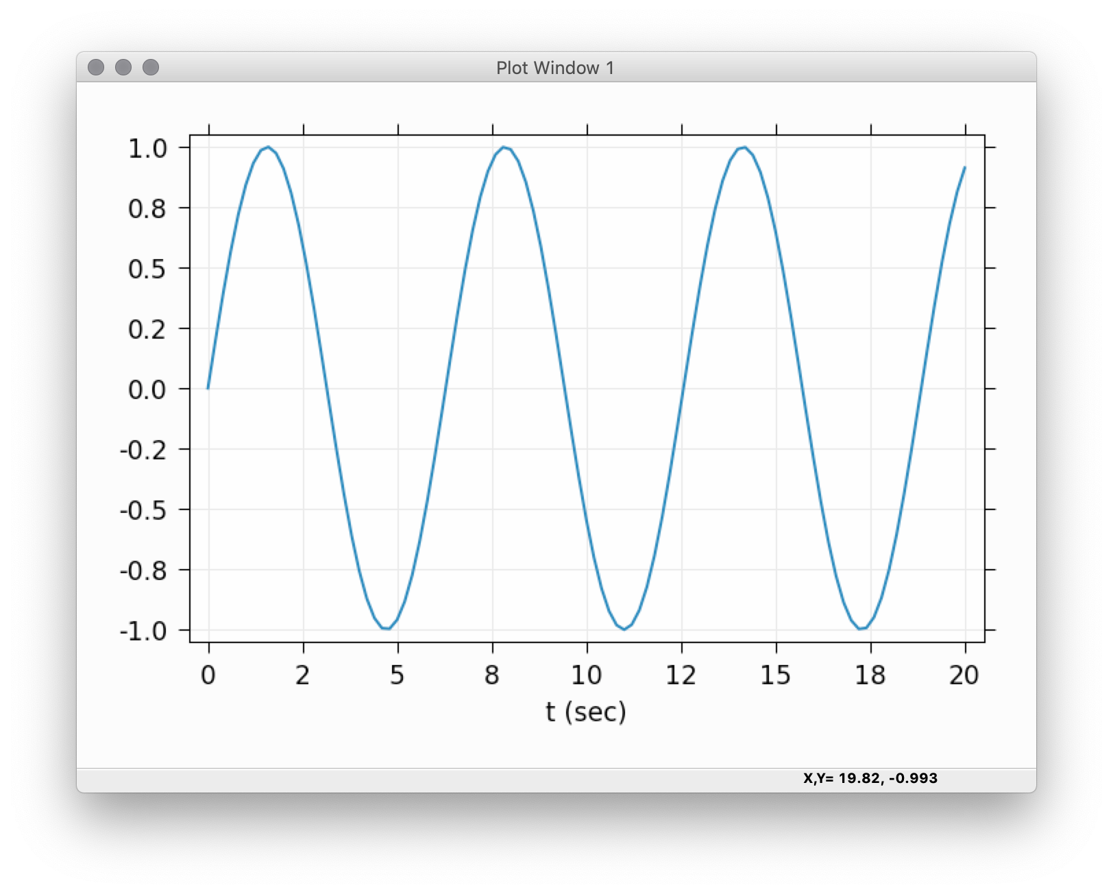
In [4]: wi.plot(x, np.sin(x), xlabel='t (sec)')
Out[4]: <wxmplot.interactive.PlotDisplay at 0x10db88678>

In [5]:

At this point a plot like this will be displayed:

As with using %matplotlib notebook in a Jupyter notebook, the wxmplot display can be zoomed in and out, but as shown in wxmplot Overview, it can also be configured and updated in many more ways.

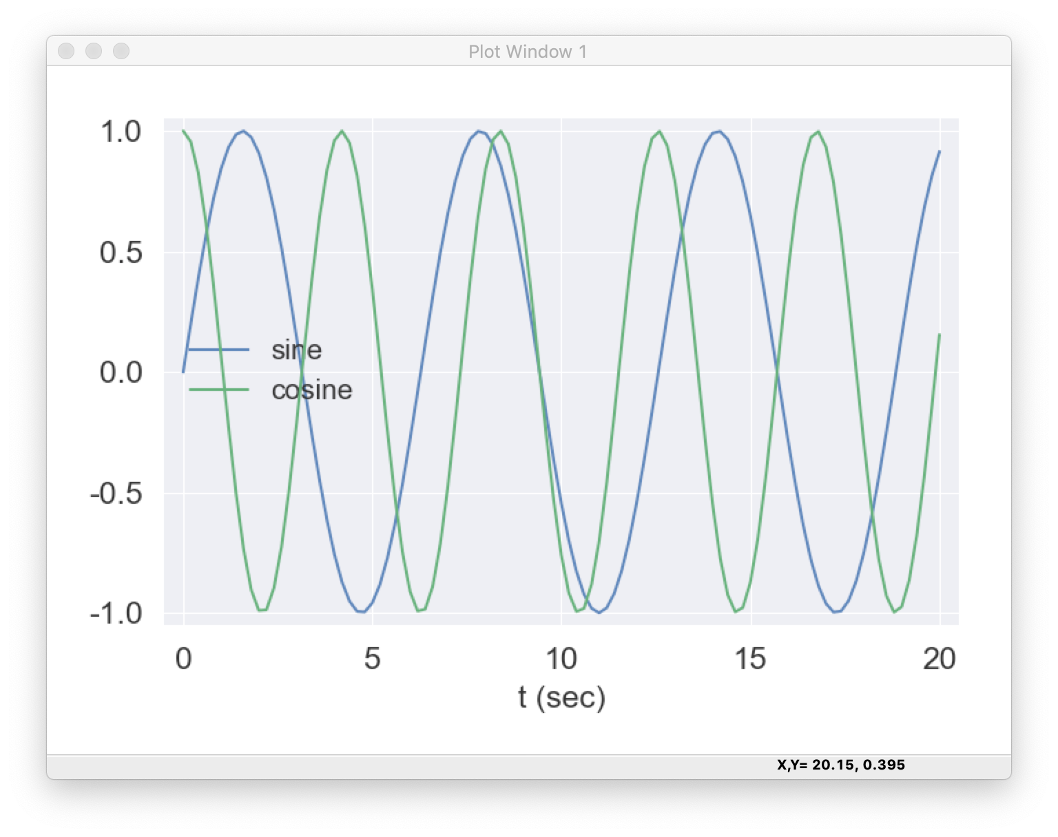
For example, from the Plot Configuration window we could change the theme to ‘Seaborn’ and set the label for this trace to be ‘sine’. Then from the Jupyter console we can continue:

In [5]: wi.plot(x, np.cos(1.5*x), label='cosine', show_legend=True)
Out[5]: <wxmplot.interactive.PlotDisplay at 0x10db88678>

In [6]:

which will now show:

which is again a fully interactive and configurable display. For example, with the legend displayed, clicking on any of the labels in the legend will toggle the display of that curve. If we want to clear the data and plot something new, we might do something like:

In [6]: wi.plot(x, x*np.log(x+1), label='xlogx', new=True)
Out[6]: <wxmplot.interactive.PlotDisplay at 0x10db88678>

In [7]:

We can also place a text string, arrow, horizontal, or vertical line on the plot, as with:

In [7]: wi.plot_text('hello!', 9.1, 0.87)

In [8]:

and so forth.

If we wanted to bring up a second 2D Line Plot window, we can use the win=2 option:

In [8]: wi.plot(x, np.sin(x)*np.exp(-x/8) , win=2, theme='ggplot')
Out[8]: <wxmplot.interactive.PlotDisplay at 0x110b2fb88>

In [9]:

and then control which of the displays any additional plot functions use by passing the win option to the plotting functions.

The immediacy of the rendering and the ability to customize the plots makes these plotting functions well-suited for exploratory displays of data.

Using the interactive functions from a script

When using the interactive functions by running a script in a non-interactive way, the display will still appear. It does not block further execution of the script and the display does not disappear when the script is complete. Instead, the plots and images will remain displayed and fully operational until all windows have been closed or until the running script is explicitly closed with Crtl-C. That means that you can add wi.plot() and wi.imshow() to your short- or long-running scripts and the plots will be displayed until you no longer want to use them.

2D Plotting with plot() and related functions

plot(x, y, win=1, new=False, ...)

Plot trace of x, y arrays in a PlotFrame

Parameters

• x (array-like) – ordinate values

• y (array-like) – abscissa values (x and y must be same size!)

• dy (array-like) – array for error bars in y (must be same size as y!)

• new (bool) – whether to start a new plot [False]

• win (int) – index of Plot Window [1]

• label (str or None) – label for this trace

• linewidth (float) – width of line joining points [from theme]

• color (str or None) – color for trace (see note 1) [from theme]

• style (str or None) – line style for joining points (see note 2)

• marker (str on None) – symbol to draw at each point (see note 3)

• markersize (float) – size of marker

• zorder (float or None) – zorder (depth) of this trace

• drawstyle (str or None) – style for joining line segments (see note 4)

• xmin (float or None) – minimum x value for plot range

• xmax (float or None) – maximum x value for plot range

• ymin (float or None) – minimum y value for plot range

• ymax (float or None) – maximum y value for plot range

• use_dates (bool) – whether to interpret x data as dates [False]

• side (str) – side for y-axis (‘left’ or ‘right’) [‘left’]

• size (tuple or None) – width, height in pixels of Plot Window

• wintitle (str or None) – title for window frame

• theme (str on None) – plotting theme to use

• title (str or None) – plot title

• xlabel (str or None) – label for x-axis

• ylabel (str or None) – label for y-axis

• y2label (str or None) – label for y2-axis (that is, right-side axis)

• xlog_scale (bool) – whether to show x-axis as log-scale [False]

• ylog_scale (bool) – whether to show y-axis as log-scale [False]

• grid (bool) – whether to draw background grid [True]

• show_legend (bool or None) – whether to show legend [False]

• legend_loc (str) – location for legend (see note 5) [‘best’]

• legend_on (bool) – whether legend is within the main axes [True]

• bgcolor (str on None) – color of background plot area (from theme)

• framecolor (str on None) – color of outer frame area (from theme)

• gridcolor (str or None) – color of grid (from theme)

• labelfontsize (float) – size (pixels) of font for Labels (from theme)

• legendfontsize (float) – size (pixels) of font for Legend (from theme)

• titlefontsize (float) – size (pixels) of font for Title (from theme)

• axes_style (str) – control what parts of axes are shown (see note 6)

• viewpad (float or None) – percent of data range to expand view ranges

• delay_draw (boole) – whether to delay drawing [False]

Returns

plotter, a PlotFrame

Notes

1. colors can be names such as ‘red’ or hex strings ‘#RRGGBB’. by default, they are set by the theme

2. styles can be one of ‘solid’, ‘short dashed’, ‘dash-dot’, ‘dashed’, ‘dotted’, ‘long-dashed’.

3. markers can be one of ‘no symbol’, ‘o’, ‘+’, ‘x’, ‘square’, ‘diamond’, ‘thin diamond’, ‘^’, ‘v’, ‘>’, ‘<’, ‘|’, ‘_’, ‘hexagon’, ‘pentagon’, ‘tripod 1’, or ‘tripod 2’

4. drawstyle can be one of ‘default’, ‘steps-pre’,’steps-mid’, or ‘steps-post’.

5. legend_loc can be one of ‘best’, ‘upper right’ , ‘lower right’, ‘center right’, ‘upper left’, ‘lower left’, ‘center left’, ‘upper center’, ‘lower center’, ‘center’

6. axis_style can be one of ‘open’, ‘box’, ‘bottom’.

More details of Plot Options are given in Table of Plot Arguments.

hist(x, bins=10, win=1, new=False, size=None, force_draw=True, title=None, *args, **kws)

display a histogram

Parameters

• x (array-like) – array of values

• bins (int) – number of bins to show

• win (int) – index of plot window

update_trace(x, y, trace=1, win=1, **kws)

update a plot trace with new data, avoiding complete redraw This can significantly descrease drawing time:

Parameters

• x (array-like) – ordinate values

• y (array-like) – abscissa values (x and y must be same size)

• trace (int) – which plot trace to update [1]

• win (int) – index of Plot Window [1]

• side (str) – side for y-axis (‘left’ or ‘right’) [‘left’]

plot_setlimits(xmin=None, xmax=None, ymin=None, ymax=None, win=1)

set plot view limits for plot in window win

Parameters

• xmin (float) – minimum x value

• ymax (float) – maximum x value

• ymin (float) – minimum y value

• ymax – maximum y value

• win (int) – index of plot window

plot_text(x, y, text, win=1, options)

add text at x, y coordinates of a plot

Parameters

• text (str) – text to draw

• x (float) – x position of text

• y (float) – y position of text

• win (int) – index of plot window

• rotation (str or float) – text rotation. angle in degrees or ‘vertical’ or ‘horizontal’

• ha (str) – horizontal alignment (‘left’, ‘center’, ‘right’)

• va (str) vertical alignment ('top', 'center', 'bottom', 'baseline') –

• side (str) – which axis to use (‘left’ or ‘right’) for coordinates.

plot_arrow(x1, y1, x2, y2, win=1, **kws)

draw arrow from x1, y1 to x2, y2.

Parameters

• x1 (float) – starting x coordinate

• y1 (float) – starting y coordinate

• x2 (float) – ending x coordinate

• y2 (float) – ending y coordinate

• side (str) – which axis to use (‘left’ or ‘right’) for coordinates.

• shape (str) – arrow head shape (‘full’, ‘left’, ‘right’)

• color (str) – arrow color (‘black’)

• width (float) – width of arrow line (in points. default=0.0)

• head_width (float) – width of arrow head (in points. default=0.05)

• head_length (float) – length of arrow head (in points. default=0.25)

• overhang (float) – amount the arrow is swept back (in points. default=0)

• win (int) – index of plot window

plot_marker(x, y, marker='o', size=4, color='black')

draw a marker at x, y

Parameters

• x (float) – x coordinate for marker

• float) (y) – y coordinate

• marker (str) – symbol to draw at each point (see Note 1)

• size (float) – marker size [4]

• color (str) – marker color [‘black’]

• win (int) – index of plot window

Notes

1. marker can be one of (‘+’, ‘o’, ‘x’, ‘square’, ‘diamond’, ‘thin diamond’, ‘^’, ‘v’, ‘>’, ‘<’, ‘|’, ‘_’, ‘hexagon’, ‘pentagon’, ‘tripod 1’, or ‘tripod 2’)

plot_axhline(y, xmin=None, ymin=None, **kws)

plot a horizontal line spanning the plot axes

Parameters

• y (float) – y position of line

• xmin (float) – starting x fraction (window units – not user units!)

• xmax (float) – ending x fraction (window units – not user units!)

• win (int) – index of plot window

plot_axvline(y, xmin=None, ymin=None, **kws)

plot a vertical line spanning the plot axes

Parameters

• x (float) – x position of line

• ymin (float) – starting y fraction (window units – not user units!)

• ymax (float) – ending y fraction (window units – not user units!)

• win (int) – index of plot window

Displaying images with imshow() and contour()

imshow(map, ...)

Display an 2-D array of intensities as a false-color map

Parameters

• map (ndarray) – map array data (see Note 1)

• y (array-like) – values for pixels along vertical direction

• x (array-like) – values for pixels along horizontal direction

• colormap (str) – name of colormap to apply

• win (int) – index of Image Window (1 to %d)

• size (tuple) – width, height in pixels of Image Window

• wintitle (str) – text for Window title [Image Window N]

• xlabel (str) – label for horizontal axis [‘X’]

• ylabel (str) – label for horizontal axis [‘Y’]

• style (str) – display style (‘image’ or ‘contour’) [‘image’]

• nlevels (int) – number of levels for contour

• contour_labels (bool) – whether to show contour labels [True]

• show_axis (bool) – whether to shos Axis [False]

• contrast_level (float) – percent level for contrast [0]

Returns

img, an ImageFrame

Notes

1. the map data can either be a 2d array (shape NY, NX) for single-color map or (NY, NX, 3) array for an RGB map

contour(map, ...)

Display an 2-D array of intensities as a contour plot

Notes

This is equivalent to imshow(map, …, style=’contour’)

Functions for working with the interactive windows

set_theme(theme)

set plotting theme by name with a theme name

Parameters

theme (str) – name of theme

Returns

None

Notes

1. Example themese are:’light’, ‘dark’, ‘white-background’, ‘matplotlib’, ‘seaborn’, ‘ggplot’, ‘bmh’, ‘fivethirtyeight’. 2. See available_themes() for the list of available themes.

available_themes()

list of available theme

Returns

list of theme names.

Notes

As of this writing, the list is:

‘light’, ‘dark’, ‘white-background’, ‘matplotlib’, ‘seaborn’, ‘ggplot’, ‘bmh’, ‘fivethirtyeight’, ‘grayscale’, ‘dark_background’, ‘tableau-colorblind10’, ‘seaborn-bright’, ‘seaborn-colorblind’, ‘seaborn-dark’, ‘seaborn-darkgrid’, ‘seaborn-dark-palette’, ‘seaborn-deep’, ‘seaborn-notebook’, ‘seaborn-muted’, ‘seaborn-pastel’, ‘seaborn-paper’, ‘seaborn-poster’, ‘seaborn-talk’, ‘seaborn-ticks’, ‘seaborn-white’, ‘seaborn-whitegrid’, ‘Solarize_Light2’

get_wxapp(redirect=False, clearSigInt=True)

get the wx App

Parameters

• redirect (bool) – whether to redirect output that would otherwise be written to the Console [False]

• clearSigInt (bool) – whether to clear interrupts of Ctrl-C [True]

Returns

a wx.App instance

get_plot_window(win=1, size=None, wintitle=None, theme=None)

return a plot display

Parameters

• win (int) – index of Plot Window (1 to 100)

• size (tuple) – width, height in pixels of Plot Window

• wintitle (str) – text for Window title [Plot Window N]

• theme (str) – theme for Plot Window [‘light’]

Returns

diplay, a wxmplot PlotFrame.

Notes

this will either return the existing PlotFrame for the window index or create a new one.

The returned wx.PlotFrame will have the heirarchy of attributes described in the table below. This allows access to the underlying matplotlib Axes and Canvas objects.

Table of PlotFrame attributes

name	object type
.panel	wxmplot.PlotPanel, a wx.Panel
.panel.conf	wxmplot.PlotConfig
.panel.axes	matplotlib.axes.AxesSubPlot
.panel.fig	matplotlib.figure.Figure
.panel.canvas	matplotlib.backends.backend_wxagg.FigureCanvasWxAgg

get_image_window(win=1, size=None, wintitle=None)

return an image display

Parameters

• win (int) – index of Image Window (1 to 100)

• size (tuple) – width, height in pixels of Image Window

• wintitle (str) – text for Window title [Image Window N]

Returns

diplay, a wxmplot ImageFrame.

Notes

this will either return the existing ImageFrame for the window index or create a new one.

As with wx.PlotFrame, the returned wx.ImageFrame will have the same principle attributes to access the matplotlib Axes and Canvas objects.