2.2 File

In MCA Disply, under File, there are the following options:

Foreground

Background

Swap Foreground <-> Background

Save Next = Filename

Save As…

New MCA Window

Print…

Preferences…

Exit

2.2.1 Foreground, Background, and Swap

A very neat aspect of this MCA widget is that you can overlay two spectra on top of each other, allowing easier comparison of data collected from two different samples. That's what Foreground and Background allow you to do. A neat thing you could do here, for example, would be to have a saved spectrum displayed in the background while a new spectra is being collected from the aim module. Both Foreground and Background allow you to collect data (if you choose Open Detector) or display an existing file (if you choose Read File). They can be swapped (Swap Foreground <-> Background).

To use either foreground or background to collect data from the aim module, select Open Detector, and you will be asked to enter the detector name. For 13-BMD, enter 13BMD:aim_adc1, whereas for 13-IDD, 13IDD:aim_adc1.

2.2.2 Save Next and Save As…

Save Next = <Filename> gives you the file name (Filename) to be used if you choose to let MCA to automatically save the data displayed on the screen. This is convenient when you have set up the file name and want save the data files in a sequence of files. See LVP file naming conventions for details on data file structure. For example, If your first data file in the current run is T0888.001, Save Next will automatically save the next file as T0888.002. Note: the file name <Filename> is the name for the data file TO BE saved, and NOT the last saved file name.

The Save As… option allows you to enter a new name for the data file to be saved.

2.2.3 New MCA Window

New MCA Window lets you open a new MCA window with various sizes.

2.2.4 Print…

Print… allows you the plot the data displayed on the MCA to a printer. The popup looks like:

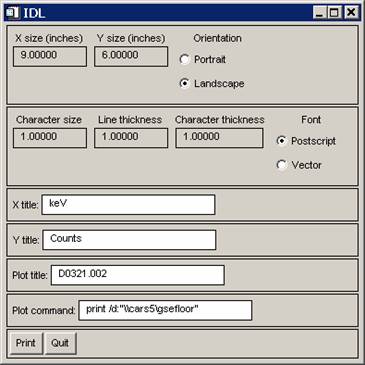
You can change the size of the plot by changing the X size and Y size parameters. You can also select portrait or landscape.

You may want to enter an appropriate title for the plot, such as “D0321.002”. Make sure plot command is “print /d:\\cars5\gsefloor”.

Click the Print button, the diffraction pattern will be plotted.

Printer Setup

Note: If necessary, you’ll have to check the setup if the above printing command does not work. In the printers directory, make sure the printer you want to use is installed.

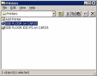
Right-click printer name, then go to Properties.

Click Sharing.

Note printer share name, “GSEFLOOR”

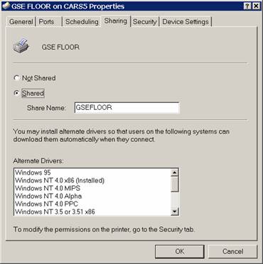
Note the plot command to print spectrum to printer "gse floor ps".

2.2.5 Preferences

Preferences… allows you to change the preferences for the MCA; it opens the following popup window:

The meaning of the various choices is self-explanatory. Choose Yes to activate the choice. Particularly, you have an option to let MCA Display to automatically save the data. This is useful when you set up the MCA to collect a series of data files at a fixed pressure and temperature condition (such as in kinetics or other time resolved experiments). By selecting yes for “Autosave when acquisition stops”, MCA will collect data for a prescribed presets time (see Controls), stop data collection, save the data in the file sequence as defined by the Save Next option, erasing the data from the MCA, and start a new data collection. You may select yes for “Informational popup after saving file”, so that you will be informed every time a data file is saved.