1.9 LVP Electronics

This section contains all electronics used for controlling the LVP operation on 13-BM-D. Click on the LVP Electronics button, you’ll see the following items.

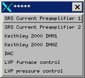
1.9.1 SRS (Stanford Research Systems) Current Preamplifier 1 is an amplifier for operations other than the LVP (e.g., DAC, tomography etc.). You won’t need to worry about this one.

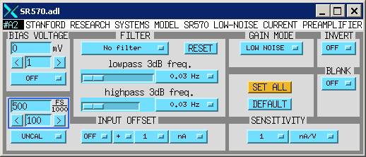
SRS Current Preamplifier 2 (Model SR 570) leads you to the following window to change setup parameter for the amplifier, which is used for transporting signals from the photo diode to the EPICS control system.

Typical parameters used for this application is shown on the right. The one parameter you’ll most likely need to change is sensitivity. Depending on the intensity of the signal, you may need to use mA/V, or pA/V. Or you may use10 nA/V; in that case just change the number from 1 to 10.

1.9.2 Keithley 1

We use two Keithley multimeters to transport analog signals for pressure, ram displacement, thermocouple emf, and heater voltage and amps, etc. All DC signals are transported through Keithley #1, wjereas AC signals through Keithley #2.

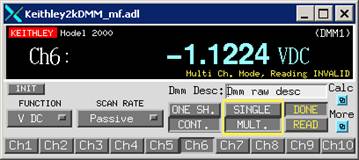
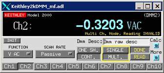
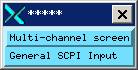
When you click on “Keithley 1”, you’ll first get a window as shown on the left. This is a single channel screen and not convenient for multiu-channel application. If you click on the small blue button on the lower right, indicated “More”, you’ll get a small window like this:

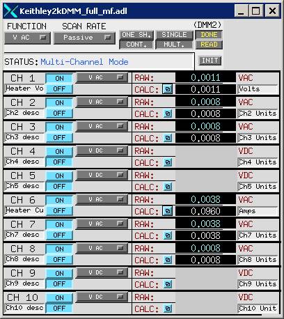
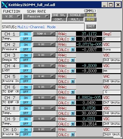Where you’re given two choices. Click the Multi-channel screen button to get to the multi-channel screen shown to your right. You’ll see there are ten channel available to you. Our current setting is summarized in the table below:

Channel	Use	Value used	Unit
1	Room T	Raw*	°C
2	Ram load	Calc**	Ton
3	--	--	--
4	LVDT	Raw	mm
5	--	--	--
6	TC emf	Calc	mV
7	TC emf	Calc	mV
8	Sample T	Calc	°C
9	Sample T	Calc	°C
10	--	--	--

Note:

* indicates raw values (i.e., values directly obtained from the channel in the Keithley

** indicates calculated value, where a mathematical transformation is performed with an algorithm defined in the Calc table for that channel.

First note that the Keithley is set for “DC” (this is done by selecting DC in the pull-down menu labeled “Function”). You may need to click the “INIT” button to start scanning all the channels. However, before doing that, you’ll need to specify a scan rate – use the pull-down menu under “SCAN RATE” to select the rate. A typical rate is 1 sec, which means the channels will be scanned and values passed on every 1 second.

Now let’s take a look at some of the channels and their functions:

Channel 1 reads room temperature from a K-type thermocouple that is built in the Keithley. Raw value is used, which gives temperature in C.

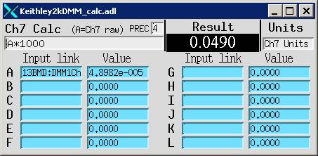
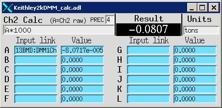
Channel 2 reads currents in mA from the pressure transducer, which ranges from 4 to 20 mA for a full pressure range up to 10,000 psi. The transducer passes on the mA to the Omega on the pressure controller, which is calibrated in kg. Thus the raw value on channel 2 is in kg, and the calculated value (raw value*1000) is in tons. This calculation is performed in Ch2 Calc (see left), where the value in field A is the raw value read from channel 2, and the calculation is defined as A*1000, as shown just under the label “Ch2 Calc”. The resultant Calc value is shown in the field labeled “Result”. Note that you can add more constants in fields B through L to define the calculation/transformation, and you can also specify precision by entering your desired number of significant digits in the field labeled “PREC”. In our case, we chose 4 digits.

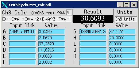
Similarly, for channel 8, where we want to pass the thermocouple emf, the raw value gives DC voltage from the thermocouple. By performing the A*1000 transformation, we’ve converted V into mV (see right). This is necessary because the thermocouple calibrations provided by the thermocouple vendors are in mV.

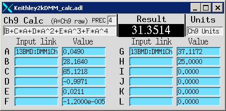
In order to calculate temperature from the thermocouple reading, we first fit the emf-temperature relationship (provided by thermocouple vendors) using a polynomial fit. For example, Channel 8 Calc screen shows a six-order polynomial fit to the D-type W/Re thermocouple (see left). In this example, field A is the value of emf from Ch 7 (if you could see the whole variable in field A, if would be “13BMD:DMM1Ch7.Calc”, which means the first digital multimeter Keithley, channel 7, calc value). Fields B through G are the coefficients of the six order polynomial fit, and the result is calculated temperature in C (30.6093), for the input emf (0.049).

Channels 6 and 7, as well as channels 8 and 9 may seem redundant. That is necessary as we use different types of thermocouples. It is useful to keep a couple sets of most commonly used thermocouple calibrations in the Keithley. Keep in mind, though, that when you want to switch thermocouples by using, say, Channel 6 instead of Channel 7, or Channel 9 instead of Channel 8, you must also remember to change the logging file catch1d.env, for it tells the MCA which parameters to log. Click this link to see details about catch1d.env.

1.9.3 Keithley 2

This is used for getting AC signals for heating. We use a 1 kW AC power supply, with several settings for heating various types of heater materials. Click here to learn the Settings of the power supply.

Keithley #2 logs heater AC voltage and current, which are then passed on to MEDM to calculate heating resistance and power. Note that the Keithley is set for AC. Although one can use one Keithley to scan both DC and AC channels, the switching between the DC and AC scanning mode takes considerable amount of time, thus slowing down the system response.

Again, you’ll get a single channel window when you click on Keithley 2. Click on the Multi-channel screen button under “more” to get to the multi-channel screen.

Only two channels are used in Keithley 2. However, we find that AC signals may “leak” to the adjacent channels. For this reason two channels next to channels 1 and 6 are shorted to prevent noise contamination. Channels 2 , 3, and 7, 8 are turned on but are only for monitoring purposes; no useful data are passed on.

For channel 1, we are interested only in the raw value (13BMD:DMM2Ch1.Raw), which is the voltage across the heater in the sample assembly. For channel 6, a calibration is used. A “doughnut” is used around one of the heating cables to sense current, and the resultant voltage cause by AC induction is 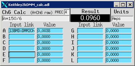calibrated using an AC Ampmeter. The raw value on Channel 6 is the voltage (A = 13BMD:DMM2Ch2.Raw), which is then used to calculate current (A*150/6).

A word about scan rate: AC scanning is based on several measured averaged over the measurement time. For this reason, one cannot expect infinite fast scan rates. In fact, any rates faster than 1 sec are unrealistic. Typical values we use are 1 or 2 seconds per scan.

1.9.4 DAC

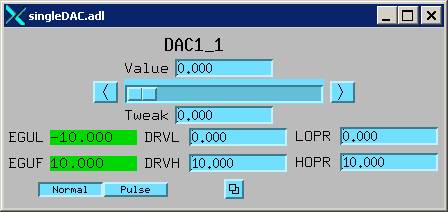
The digital-analog converter (DAC) is used to control the power supply for heating. The DAC sends a control voltage ranging from zero to 10 VDC, which conrresponds to 0 to full power (1 kW). The old way to control heating is by manually increasing the control voltage in the window shown on the left. This has been superceded by the LVP Furnace control function in Section 1.9.5.

1.9.5 Furnace control

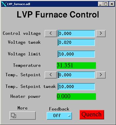
. This section describes procedures for heating and temperature control. The main furnace control window is shown on the right. Control voltage is the control signal from the DAC (see 1.9.4 above). Voltage tweak sets the step size for tweaking. In the example shown on the right, if you click the button on the right hand of the Control voltage field (with the right pointing arrow), control voltage will increase by 0.020 V (set by the tweak field), unless the control voltage has reached the upper limit. Click on the left button (left pointing arrow) will decrease the control voltage by 0.02, unless the control voltage is at the lower limit (0.000).

The absolute upper limit is 10 V; however, most times you’ll want to define a dynamic upper limit, which can be any positive value. A good practice is to change the dynamic upper limit, so that it is slightly above the control voltage, which you want to use to maintain a temperature. The advantage is that in cases where there is a power surge (either due to heater instability or environmental noise), the dynamic upper limit will be in control and the temperature will not be way off your range.

The Temp. Setpoint and Temp. Setpoint tweak are use for temperature feed back control. Note that in reality you can feed-back control not only temperature, but also power, or voltage for that matter. All you need to do is to set the Process Variable (PV) in the Temp. Setpoint field. Right click in that field and you’ll se the current PV in it. To set a new PV for feed back control, simply middle click a field that contains the new PV and drag it to the Temp. Setpoint field and then hit the enter key. You’ll need to right click the field to double check.

The green fields (Temperature and Heater power) are for display only – you won’t be able to change the values in those fields.

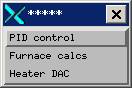
Now click on the lower left button “More” and you’ll see three choices: PID control, Furnace calcs, and Heater DAC. Heater DAC is covered in 1.9.4, and Furnace calcs is a transformation record used to calculate heater resistance 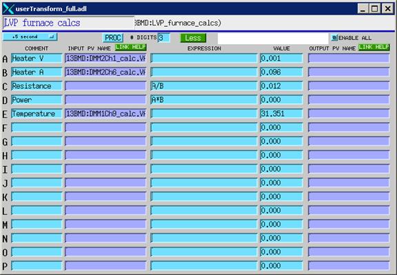and power (see left). Fields A and B are direct inputs of heater voltage and current from Keithley #2. C is calculated resistance (A/B) and D heater power (A*B). E is temperature from calculations passed on by Keithley #1. These values will be passed on to other records for monitoring or calculation purposes.

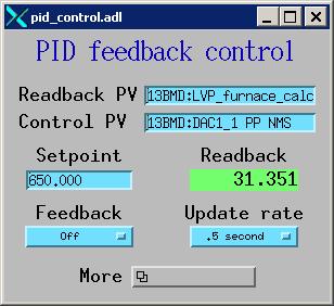The first item, “PID feedback control”, is used to set up feed back and run feedback control. The field “Readback PV” contains the PV that you want to run feedback control with. If you are running feedback on temperature, this will be the temperature value; if you are running on power, this will be the power. Control PV is always the DAC control voltage (13BMD:DAC_1).

The “Setpoint” sets the value you want to maintain and “Update rate” sets the rate for feedback update. In the example on the left, .5 second means the value will be checked and adjusted accordingly every half a second.

Note that you must consider also the update rates you set on the Keithleys. Sometimes the update rates on the keithleys are slow (e.g., 10 second) and this can cause the feedback to oscillate or even unstable, because the feedback control updates at a much faster rate to increase or decrease power then the readback from the Keithleys. If this happens, the oscillation may become bigger and bigger over time.

Like in the main control window, the green field is for viewing only. However, you can change the PV so that the desired values are shown in this field. For example, if you are running power control, you should enter the PV for heater power.

The feedback button allows you to turn the feedback on or off.

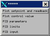
The “More” button gives you five options, shown on the right. These options allow you to modify PID parameters and to plot setpoint and feedback values to visualize the quality of the feedback control.

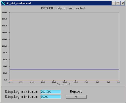
The “Plot setpoint and readback” button gives visual display (left) for the setpoint and feedback values. In this plot, the current time is always on the right (0.0) and the values in the past 30 seconds are plotted towards left. You can set the minimum and maximum vertically to plot the data. Note that the Replot button does not work properly right now – i.e., clicking Replot after changing the Display maximum and/or minimum does not rescale the plot. What you’ll need to do right now is to re-size the window.

The “Plot control value” button will plot the control values (e.g., DAC).

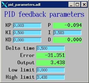
The PID parameters button opens the window for “PID feedback parameters”. The PID uses three terms to control the feedback: proportional, integrated, and derivative. An detailed description of the GSECARS extended PID control process is given by Mark Rivers and can be found here.

For our applications with TiC/diamond heater or graphite heater, typical values of the control parameters are:

KP: 0.000 – 0.006

KI: 0.500 – 1.000

KD: usually 0

You’ll need to monitor your furnace response carefully at the beginning of the heating to find out the best combination. Also note that the DAC control voltage tweak has finite size, and sometime extremely small change in temperature may not be realistic. In addition, for the same control voltage change, temperature responses much more sensitively at high temperature than at low temperature. For this reason, generally you need to decrease the KP value as temperature increases. Around 1000C, KP is typically 0.001.

The High limit is the same as the dynamic limit you set on the Furnace Control main page.

The fourth option, “PID limits”, allows you to set up limits for heating control. Note that these limits are somewhat different from the limit we have seen on the PID feedback record and the Main LVP Furnace control record. In those records, the limit is for the control voltage only. Here the transformation record calculates limits based on a number of parameters, heater volts, current, and power. Note that heater volts are different from control volts. The latter is always 0 – 10 V, corresponding to 0 to maximum power of the supply (1000 W). Heater volt is the actual voltage across the heater. It is different from control volts: depending on the supply setting, the maximum heater voltage can be either 5, 10, 20, or 50 V, with maximum current of 200, 100, 50, and 20 Amp (making the maximum power of 1000 W). Even for the setting of 10 V/100Amp maximum, the heater volt can be different from the control volt, because the heater volt is measured from the connectors built in the pressure module upper and lower guide block, whereas the control volt is a signal sent from the DAC.

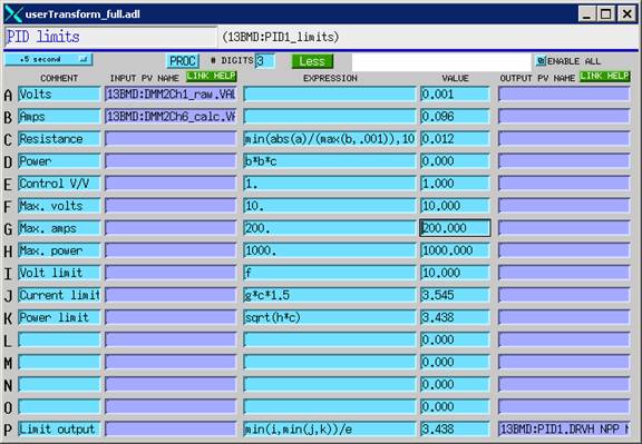
In the transformation record shown on the right, A and B fields are the measured (“real”) Volts and Amps across the furnace. C is calculated resistance (=A/B) and D calculated power (B*B*C). E is the ratio of control voltage to maximum heater voltage, which is unit for the setting of 10V/100Amp. For other settings it will be different. For example, for the setting 5V/200Amp, the control V/V value is 10/5=2. Maximum volts and amps (fields F and G) are according to the setting and maximum power is always 1000 for the power supply in 13-BM-D. Fields I, J, and K are calculated limits for Volt, Current, and Power, respectively, and are used in the PID feedback control, as long as any limit is reached, the controller will stop increasing the power. This is used to prevent run-away heating during the feedback control.

Sometimes you may want to manipulate the limits by changing either the max values (fields F, G, or H), or the limits (e.g., multiply a parameter with a constant that is either less or greater than unity (e.g., field J is multiplied by 1.5).

1.9.6 LVP Pressure Control

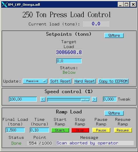The 250 Ton Press Load Control record is divided into three parts. The top part, Setpoints is for setting the target load. Enter the target load in the blue window directly under “Target Load”. This is your setpoint for pressure control. EPICS will use this value to the setpoint in the Omega controller on the pressure control box. Note that “Update” must be in seconds or fraction of seconds (typical value: 2 – 5 sec). If it is set as “passive”, then setpoint will not be in effect.

The middle part of the screen is Speed control. The maximum speed (100%) is set manually on the pressure control box mounted directly on the VME crate. Turn the pot knob clockwise to increase speed. The maximum speed is 1,800 RPM, but typical speed for increasing ram load is about 100 to 150 RPM. If the speed on the omega controller is set at 100 (RPM), then this will be the maximum speed the pressure control can automatically reach. One can choose a lower speed by changing the percentage to less than 100%.

Note that the direction control knob on the pressure control box must be turned to “INCR” in order to increase ram load. With this directional setting (INCR), you can still decrease the load, if you enter a new target load value in the Setpoints field. The speed in decreasing load is fixed at -48 RPM with this setting. For faster load decrease, you’ll need to turn the directional control knob to “DECR”.

The lower part of the screen Ramp Load is for ramp control. This will let you to define a ramp speed from the current load to the next target load (called “Final Load”) is a specified number of hours. This load range will be automatically divided into 1000 equal points, and MEDM will perform a scan operation between the initial and final load to increase or decrease the load according to the time intervals defined. Again, if you want to decrease load faster than 48 RPM, you’ll have to turn the directional knob to “DECR”.

Note: Be careful when use Ramp Control at the beginning of the run (i.e., run pressure up from zero, when there are still gaps between the guide blocks and the cell assembly. You’ll need to set the maximum ram speed no higher than the typical rate of 100 -150 RPM using the pot. To close down the gaps, the load will not increase for certain periods of time, and Ramp control may increase to speed to the maximum in order to follow the rate defined by the Time specified in the record (see below). Having a very high maximum RPM on the pressure control box may result in “hard landing” on the cell assembly, damaging the cell.

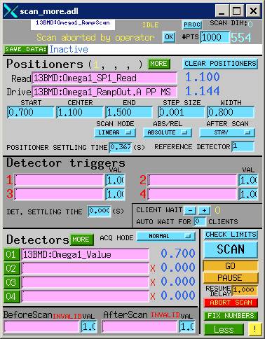
The More button on the pressure control record will bring you to the scan record, shown on the right. This is used for the ramp control, which basically divides the load range between the present value and the Final load (and the time from the beginning to the end) into 1000 setpoints, and runs a scan, i.e., it tries to increase the load to the first setpoint at the time calculated based on the number of hours you’ve specified to reach that load, by varying the ram speed. Once it reaches there, it will attempt the second setpoint, and so on. This scan record is not for other scanning purposes.

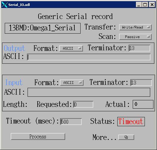
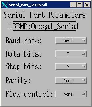
The More button under Setpoints is generally not used. It contains a Generic Serial Record which defines the input and output formats, as well as a record defining serial port parameters. Default values are shown in the images below.