
9.3. XANES Analysis: Linear Combination Analysis, Principal Component Analysis, Pre-edge Peak Fitting
XANES is extremely sensitive to oxidation state and coordination
environment of the absorbing atom, and spectral features can often be used
to qualitatively identify these characteristics. On the other hand, the
physical origin of the spectal features are complicated enough that direct
and complete quantitative analysis is difficult. As a result, “XANES
Analysis” of a spectrum typically involves making linear combinations of
spectra from known compounds or fitting the spectral features and
correlating trends in their positions and intensities to known changes in
spectral features with the desired characteristic such as oxidation state.
This approach to spectroscopy can be incredibly accurate and sensitive but
ultimately relies on comparisons to spectra of known materials. In all
cases, XANES analysis uses normalized XAFS spectra, as done with either
the pre_edge() or mback() function.
Within the context of Larch, there are two basic approaches to analyzing XANES spectra. The first of these involves fitting of the so-called pre-edge peaks that are (generally) due to hybridization of \(d\) electron bands of a transition metal with oxygen \(p\) electrons. These peaks are at energies just below the main (\(4p\) for first row transition metals) edge. They are typically split into several distinct multiplet energies corresponding to molecular orbitals of the hybridized metal \(3d\) (for firs-row transition metals) and (typically) oxygen \(2p\) orbitals. These features are quite robustly correlated with electronic and local atomic structure of the metal and its ligands, and quite a rich literature makes use of such pre-edge peak fitting in a variety of fields. As the energy resolution of XANES measurement continues to improve, thes pre-edge peaks become clearer and a richer resource for spectral analysis.
The second general approach to XANES analysis is to treat experimental XANES spectra as a linear mixture of the XANES spectra of idealized components. This works on the assumption that the XANES signature of a collection of atoms is the linear sum of the XANES from individual components, which is valid in all but the most extreme conditions. In this sense Linear Combination Analysis is a very useful approach to XANES analysis, and generally quite easy to do. If done carefully, it can also quite robust, though its sensitiviy can be somewhat limited.
What is not always clear in Linear Combination Analysis is what the proper “standard” components should be, or even how many can be determined from a collection of data. In this sense standard spectroscopic methods such as Principal Component Analysis (or PCA) and other linear-algebra based analysis tools (which are nowadays often included in “Machine Learning” methods) can be useful. Strictly speaking, PCA is very limited in what it can really tell you about a set of spectra – it helps you identify how many unique components make up a collection of spectra, and can help answer if another spectrum is also explained well by those principal components, and so “fits in” with the starting collecion of data. This is admittedly limited knowledge, but can be very useful in enabling further analysis.
These three of these approaches are exposed in the XAS Viewer application described in Chapter 4.3, and the documentation here largely reflects the operations done there.
But first a note for all XANES analysis. All these methods rely on comparing the spectral intensities normalized to the main absorption edge. Thus, in order to get accurate quantitative results, the spectra analyzed need to be well-normalized. More importantly, they need to be consistently normalized. In addition, sample preparation and measurement issues such as pinhole effects, over-absorption and detector saturation or deadtime can systematically alter the XANES spectra. None of the analytic methods described here for XANES analysis can independently identify when spectra are not properly normalized or when artifacts that suppress the spectral features have occured. It is up to the experimentalist and analyst to make these decisions.
9.3.1. Pre-edge Peak fitting
Pre-edge peaks can often be modeled as a simple sum of mathematical
functions such as gaussian(), lorentzian(), or voigt().
Typically, no more than 4 functions are needed to model most pre-edge
peaks. Still, it is not always so simple to identify several aspects of
pre-edge peak fitting. These challenges include
- identifying and removing the background due to the main absorption edge.
- identifying the proper shape of the peaks.
- making sure that the peaks overlap but do not exchange or become coincident.
The XAS Viewer application helps with each of the tasks, and it is highly recommended that you start with this GUI.
9.3.2. Linear Combination Analysis
Many XANES spectra are made on messy, heterogeneous systems or in engineered samples in which a predictable if not completely understood reaction is occuring. In these cases and many related problems, using linear combinations of spectra from known compounds to understand the makeup of the unknown sample is an important analysis method.
-
_math.lincombo_fit(group, components, weights=None, minvals=None, maxvals=None, arrayname='norm', xmin=-np.inf, xmax=np.inf, sum_to_one=True)¶ perform linear combination fitting for a group
Parameters: - group – Group to be fitted
- components – List of groups to use as components (see Note 1)
- weights – array of starting weights (see Note)
- minvals – array of min weights (or None to mean -inf)
- maxvals – array of max weights (or None to mean +inf)
- arrayname – string of array name to be fit [‘norm’] (see Note 2)
- xmin – x-value for start of fit range [-inf]
- xmax – x-value for end of fit range [+inf]
- sum_to_one – bool, whether to force weights to sum to 1.0 [True]
Returns: group with resulting weights and fit statistics
Notes:
- The names of Group members for the components must match those of the group to be fitted.
- use
Noneto use basic linear alg solution) - arrayname can be one of norm or dmude
-
_math.lincombo_fitall(group, components, weights=None, minvals=None, maxvals=None, arrayname='norm', xmin=-np.inf, xmax=np.inf, sum_to_one=True)¶ perform linear combination fittings for a group with all combinations of 2 or more of the components given
Parameters: - group – Group to be fitted
- components – List of groups to use as components (see Note)
- weights – array of starting weights (see Note)
- minvals – array of min weights (or None to mean -inf)
- maxvals – array of max weights (or None to mean +inf)
- arrayname – string of array name to be fit (see Note 2)
- xmin – x-value for start of fit range [-inf]
- xmax – x-value for end of fit range [+inf]
- sum_to_one – bool, whether to force weights to sum to 1.0 [True]
Returns: list of groups with resulting weights and fit statistics, ordered by reduced chi-square (best first)
See notes for
lincombo_fit().
9.3.3. Principal Component Analysis
To use Principal Component Analysis, you must first use a collection of spectra to build or “train” the model. With a trained model, you can ask how many independent components are needed to describe the variation in the collection.
-
_math.pca_train(groups, arrayname='norm', xmin=-np.inf, xmax=np.inf, sum_to_one=True)¶ use a list of data groups to train a Principal Component Analysis model
Parameters: - groups – list of groups to use as components
- arrayname – string of array name to be fit (see Note) [‘norm’]
- xmin – x-value for start of fit range [-inf]
- xmax – x-value for end of fit range [+inf]
Returns: group with trained PCA model, to be used with
pca_fit()- The group members for the components must match each other in data content and array names.
- arrayname can be one of norm or dmude
The trained PCA group returned will have the following members:
name meaning x x or energy value from model arrayname array name used to train model labels list of labels (filenames for each input group) ydat 2D array of input components, interpolated to x xmin minimum x value used. xmax maximum x value used. pcamodel raw return value from scikit-learn PCA.fit().mean mean value of ydat. components list of components, ordered by variance score variances list of weights for each component.
-
_math.pca_fit(group, pca_model, ncomps=None, _larch=None)¶ fit a spectrum from a group to a pca training model from pca_train()
Parameters: - group – group with data to fit
- pca_model – PCA model as found from
pca_train() - ncomps – number of components to included
Returns: None.
On success, the input group will have a subgroup name pca_result created with the following members:
name meaning x x or energy value from model ydat input data interpolated onto x yfit linear least-squares fit using model components weights weights for PCA components chi_square goodness-of-fit measure pca_model the input PCA model
9.3.4. PCA example
A simple example of using these PCA functions is given below, building on the dataset from Lengke, et al shown in section 8.6.3. Here, we’ll first read in six “standards” and one unknown spectra from an Athena project file and extract the desired groups. We then make sure that all the spectra have pre-edge subtraction and normalization done consistently. This may not be necessary if care was taken in the steps that generated the project file, but we include it here for completeness.
## examples/pca/pca_aucyano.lar
# note that this is similar to examples/fitting/doc_example3

auproject = read_athena('cyanobacteria.prj', do_fft=False, do_bkg=False)

d_720       = extract_athenagroup(auproject.d_720)
au_foil     = extract_athenagroup(auproject.Au_foil)
au_cl3aq    = extract_athenagroup(auproject.Au3_Cl_aq)
au_hydrox   = extract_athenagroup(auproject.Au_hydroxide)
au_sulfide  = extract_athenagroup(auproject.Au_sulphide)
au_thiocyan = extract_athenagroup(auproject.Au_thiocyanide)
au_thiosulf = extract_athenagroup(auproject.Au_thiosulphate_aq)

# make sure pre_edge() is run with the same params for all groups
for g in (d_720, au_foil, au_cl3aq, au_hydrox, au_sulfide, au_thiocyan, au_thiosulf):
    pre_edge(g, pre1=-150, pre2=-30, nnorm=1, norm1=150, norm2=850)
#endfor

standards = (au_foil, au_cl3aq, au_hydrox, au_sulfide, au_thiocyan, au_thiosulf)

# train model with standards
au_pcamodel = pca_train(standards, arrayname='norm', xmin=11870, xmax=12030)


# plot components and weights
plot_pca_components(au_pcamodel, min_weight=0.005)
plot_pca_weights(au_pcamodel, win=2, min_weight=0.005, ylog_scale=True)

# print out weights
total = 0
print(" Comp #  |  Weight   |  Cumulative Total")
for i, weight in enumerate(au_pcamodel.variances):
    total = total + weight
    print("  %3i    | %8.5f  | %8.5f " % (i+1, weight, total))
#endfor

# fit unknown data to model
pca_fit(d_720, au_pcamodel, ncomps=4)

# plot
plot_pca_fit(d_720, win=3)


## end of examples/pca/pca_aucyano.lar
Next, we’re ready to train the PCA model with the collection of standard spectra, so we make a list of groups standards and create a training model that we store in au_pcamodel.
With this PCA model, we can investigate the components and their weights. To be clear, the PCA process first calculates and removes the mean of all the components and then focuses on the variations in the spectra. This is especially helpful for XANES spectra as the mean normalized \(mu(E)\) is almost always larger than the variations. We can then plot the mean and the principal components themselves (in Figure 9.3.1), and the weight of each component (in Figure 9.3.2) to explain the variations in the training set (note that this does not include the mean, and is on a log scale).
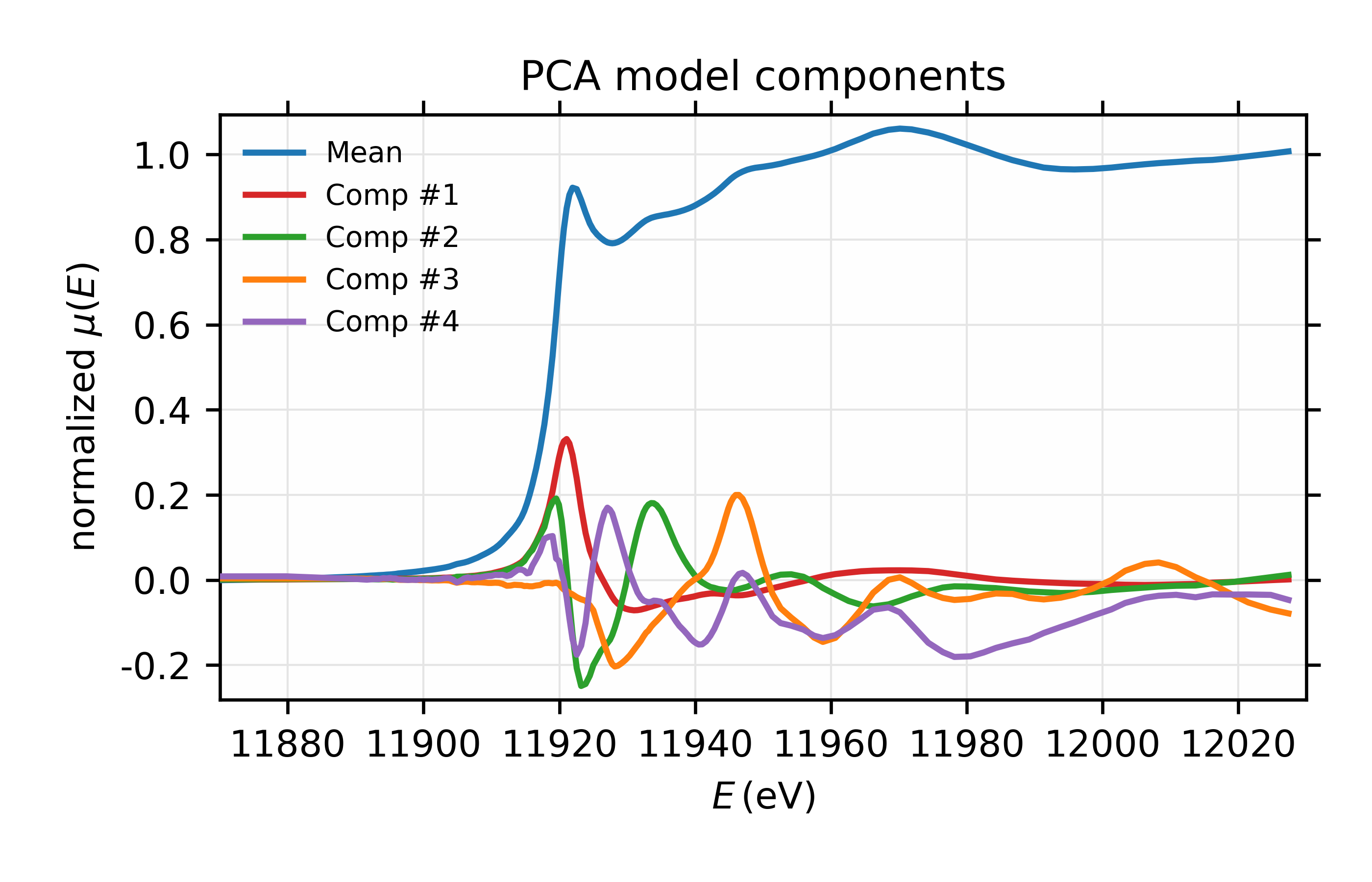
Figure 9.3.1 Mean and 4 most important components.
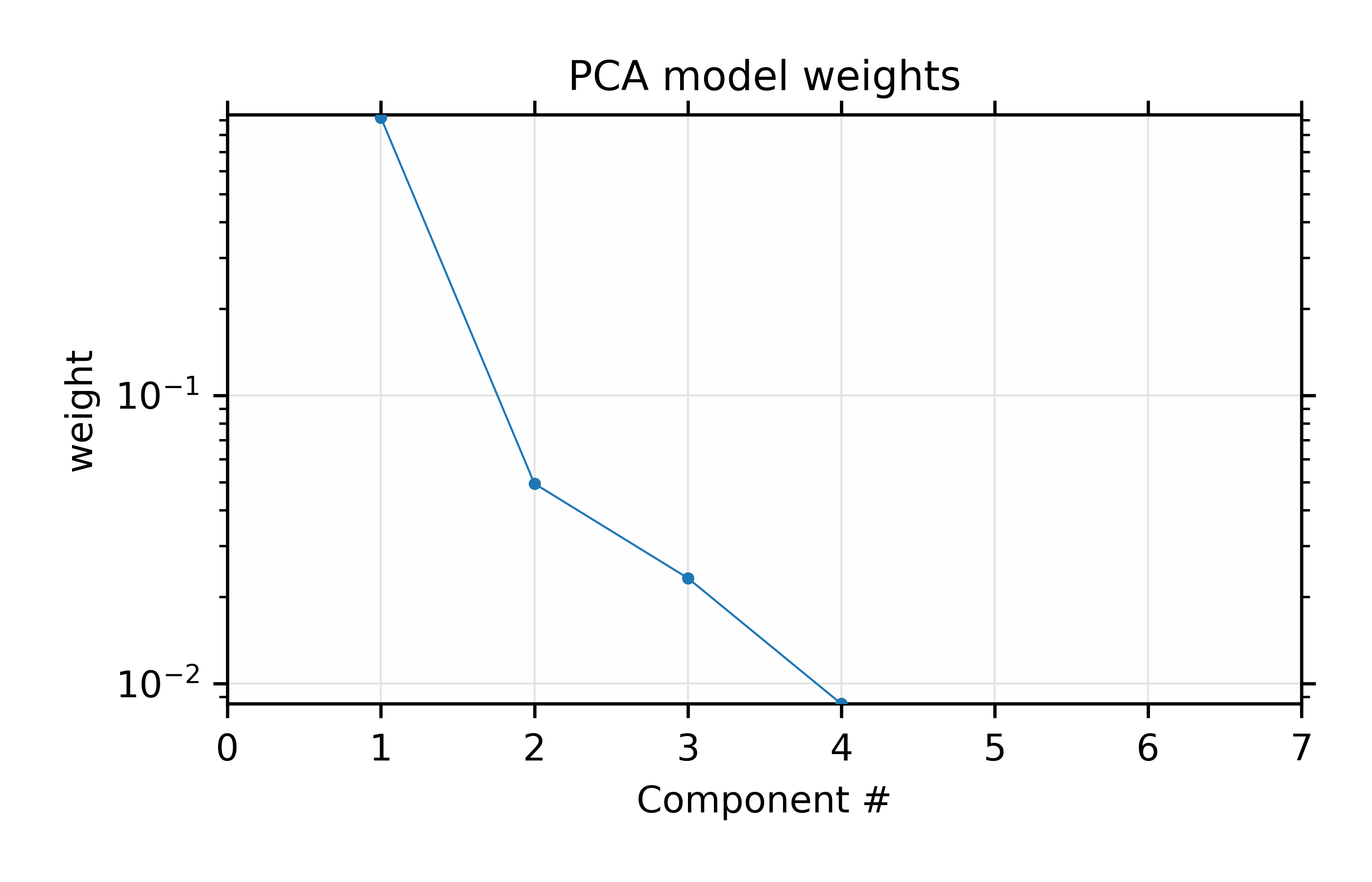
Figure 9.3.2 Fractional weights or variances for the 4 most important components of the Au XANES spectra – not including the mean spectrum.
Results for the PCA training set of 6 Au \(L_{III}\) XANES spectra.
We also print out the weights of the components which will give:
Comp #  |  Weight   |  Cumulative Total
   1    |  0.91834  |  0.91834
   2    |  0.04938  |  0.96772
   3    |  0.02321  |  0.99093
   4    |  0.00850  |  0.99942
   5    |  0.00058  |  1.00000
   6    |  0.00000  |  1.00000
which shows the values for the weights plotted in Figure 9.3.2 for the principal components. This shows that the first 2 components explain 95% of the variation, and that using 4 components will explain 99.9% of the variation in the data.
Finally, we finish the example script by seeing if the unknown spectrum can be explained by the 4 principal components from the training set. This is shown in Figure 9.3.3 and gives good confidence that the data should be able to be explained by 4 components. This is consistent with the findings using linear combination analysis in section 8.6.3, but gives a slightly firmer foundation for using that number of components.
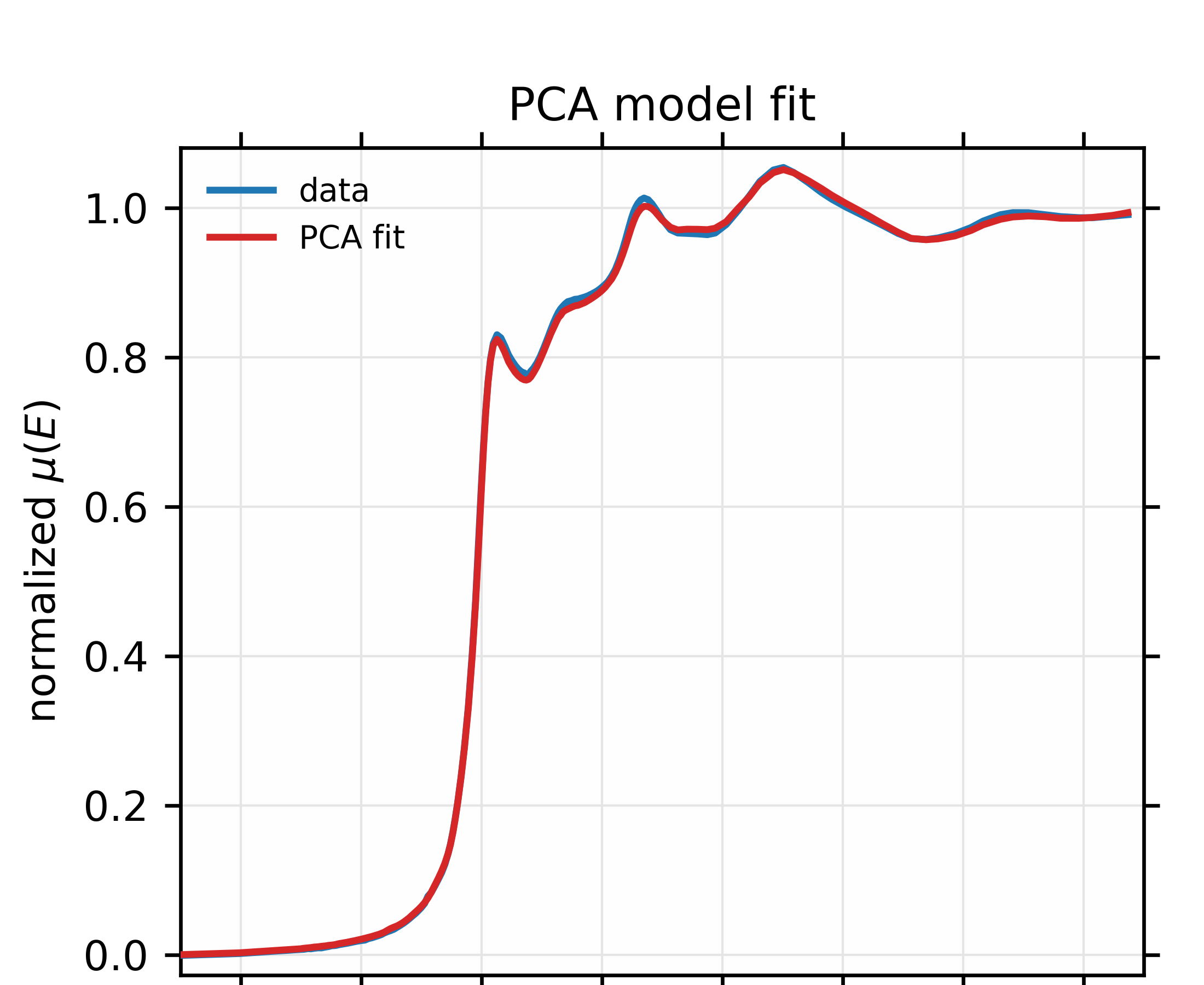
Figure 9.3.3 Fit to unknown Au \(L_{III}\) XANES spectrum to a linear combination of the mean and 4 principle components of the training set. The fit looks good enough to conclude that this spectrum probably is explained by the variances seen in the main 4 components from the training set.